


Introduction
After seeing transformers taking over natural language processing and then image classification with ViT, dense image prediction tasks were the next in line to fall. Traditionally, tasks like depth estimation (regressing a depth value for each pixel) and semantic segmentation (assigning a class label to every pixel) have relied on convolutional networks, often structured as encoder-decoder architectures like U-Net.
While very effective in low-data regimes, these designs face limitations since progressive downsampling erodes thin spatial details that aren’t always recoverable, and the local receptive field of convolutions delays global context modeling until the very last layers.
The Dense Prediction Transformer (DPT) [1] challenges this status quo, bringing high-resolution and globally coherent outputs to the table with an architecture that, to some extent, still carries forward the legacy of the U-Net. Let’s dive in!
Architecture
Let’s arrive at DPT by starting from a U-Net (covered in #17), maybe simulating the thought process of the authors. We want to transfer its encoder-decoder structure, skip connections, and the idea of seamlessly assembling multi-resolution features at various levels.

Step 1: Vision Transformer as encoder
The convolutional layers in the U-Net encoder are nothing but hierarchical feature extractors. What typically happens is that due to memory requirements, the deeper we go, the more we trade spatial resolution for richer semantic features at the cost of some fine details.
If we use a ViT [2] encoder, which operates at a constant resolution, this is no longer the case. After we flatten the input image into non-overlapping patches (e.g., 16×16 pixels) and embed each patch as a visual token, we end up at the other end of the transformer with the same number of tokens and with the same embedding dimension (e.g., 768). Same if not better semantic features, but no unnecessary compression happening.
Crucially, every token can attend to every other token right from the very first layer. This means ViT maintains a global receptive field throughout the entire network, and as you can imagine, this is a big deal for dense prediction tasks that demand continuous reasoning over spatial relationships in the scene (e.g., near and far planes in depth). Encoder swapped, next is the decoder.

Step 2: Reassembling tokens into spatial features
U-Net propagates intermediate feature maps from the encoder directly into the decoder, allowing it to recover some spatial detail that might otherwise get lost at the bottleneck. But now that our encoder is a Vision Transformer, it outputs the same flat sequence of tokens after each transformer block, not a “structured” feature map.
To decode and assemble them into an image-like output, we first need to reintroduce spatial structure. However, there is an additional complication coming from the “readout” token that needs to be addressed. In standard ViT, a special extra token T₀ is prepended to the image patch tokens (T₁, …, Tₙ), with the idea that this token does not correspond to any spatial location in the input and so can focus on useful global information (e.g., predict the label in image classification).
So, when reassembling tokens into spatial maps, we first need to decide what to do with the readout token. The authors analyze three strategies to deal with it:
Discard it entirely.
Add it back to every spatial token via element-wise addition (T₁ + T₀, …, Tₙ + T₀).
Concatenate it to each spatial token and pass the result through a projection layer to restore the original dimension (MLP(cat(T₁, T₀), …, MLP(cat(Tₙ, T₀)). This is what seems to work best, at the cost of more parameters.
At this point, at selected transformer layers, we can reshape back into 2D grids the tokens (e.g., for a 224×224×3 input with 16×16 patches, that would be a big 14×14×768 tensor). After this, a set of “Reassemble” convolutions follows, reducing the number of channel dimensions and adjusting the spatial resolution either via upsampling or downsampling, so that it matches the scale expected at each stage of decoding.

This process is repeated for four different layers of the transformer. In the case of ViT-Base with 12 layers, these are layers 3, 6, 9, and 12. The result is a set of spatial feature maps at multiple resolutions, which will be combined by the decoder for refinement. Cool, now we also have the equivalent of the “multi-scale future maps” of the U-Net!
Step 3: Decode
Once the feature maps have been reassembled into image-like tensors, they are passed into a cascade of fusion blocks, each consisting of convolutional units and upsampling layers. Fusion proceeds step-by-step, merging low-resolution semantic features from the deeper layers with the high-resolution spatial details extracted by the first ones.
The fusion blocks include residual connections (the “Residual Conv Units” in the diagram), making DPT variants easy to optimize, also due to the relatively shallow and light decoder. And that’s it, we have completed our journey from a 2015 U-Net to a 2021 DPT! What is left to do is attach a simple task-specific classification/regression head based on the desired dense prediction objective and train.
Applications and rationale
The embedding layer in a ViT projects each image patch into a high-dimensional vector space. Crucially, the space dimension is larger than the number of pixels in a patch. For example, a 16×16 patch has 256 pixels, but is typically mapped to a 768- or 1024-dimensional embedding.
This means that the embedding procedure (and the encoder itself), by design, isn’t strictly bottlenecked by dimensionality. The ViT encoder is a wide learning highway capable of preserving all sorts of fine-grained spatial information during patch projection, if doing so is beneficial for solving the problem.
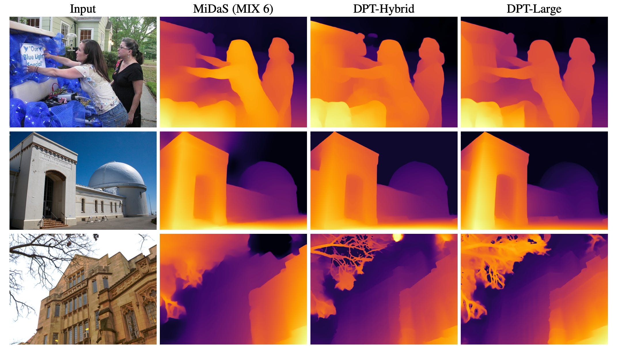
This property makes DPT a formidable model when both global context and memory of fine details in the input are required to perform at the top. When DPT was introduced, it delivered an average zero-shot depth estimation improvement of 28% compared to its predecessor, MiDaS [3]. This is attributed to the good design properties, but also the capacity to train on much more data without bottlenecks.
Conclusions
DPT reimagines the classic U-Net architecture around the Vision Transformer, and achieves the rare combination of fine spatial details, global consistency, and efficient inference. With model capacity no longer a limiting factor, the real deal shifts back to the quality and quantity of training data, which is still relatively scarce compared to text or image datasets.
ViTs are data-hungry, and if we take depth estimation as an example, they are still improving to this day, powered by synthetic data and even pseudo-predictions from other models or larger ViT variants.
If you want to try DPT in your next project, it was recently added to the Segmentation Models Pytorch [4] library, the place to go for plug-and-play segmentation. What happened from here? Well, there is another, arguably cooler, approach to tackling dense prediction tasks: diffusion. We’ll dive into that soon. See you next week!
References
[1] DPT: Vision Transformers for Dense Prediction
[2] ViT: An Image is Worth 16x16 Words