
32. I-JEPA
Self-supervised learning on images with a joint-embedding predictive architecture


Introduction
Throughout our journey into self-supervised learning for images, we have seen a significant evolution in the techniques advancing this field. Starting with contrastive learning and negative pairs in SimCLR (#6), we progressed to multi-view consistency approaches in BYOL (#11) and DINO (#15), shifted to token prediction in BEiT (#19), and eventually landed on patch-based reconstruction in Masked Autoencoders (#24).
With every paper, we progressed toward better label-free pretraining, and at the same time, saw a gradual abandonment of complex augmentations and handcrafted priors. If SimCLR relied heavily on cropping, color augmentations, and large batches with negatives, later methods started to learn more directly from raw visual signals, using fewer tricks, a single image, and ultimately even a single view.
Today, we are ready to discuss I-JEPA [1], or Image Joint Embedding Predictive Architecture, introduced by Meta AI in 2023 as the first concrete expression of Yann LeCun’s vision for more human-like AI. This new paradigm for learning features from unlabeled images (and more) is focused on efficiency, scaling, and forecasting high-level image representations rather than low-level details. Let’s go through it!
The problem with pixel reconstruction
As we discussed in the context of MAEs, learning by filling in the blanks works, but comes at a cost when applied to images: the model ends up focusing on low-level details that are irrelevant for downstream tasks. Resulting features underperform in evaluation settings such as linear probing and require more involved end-to-end fine-tuning to achieve state-of-the-art performance.
Think about this: if we are predicting a patch of sky based on context, do we really need to know whether it is blue or grayish? Or is it enough to understand that it is indeed sky? From the perspective of most downstream tasks, the semantic category and the concepts are what matter, not the exact pixel values.
Therefore, the focus shifts back to predicting latent representations (more abstract, efficient, and useful), while building on the core strengths introduced by MAE:
The use of a single input view
Masking as a learning objective
The architectural advantages of a fully vision transformer-based setup, e.g., processing only a subset of patches in the encoder.
The result is a big surge in the quality of the frozen features, reflected in linear probing evaluation, as well as improved training speed and scaling trend.
Method
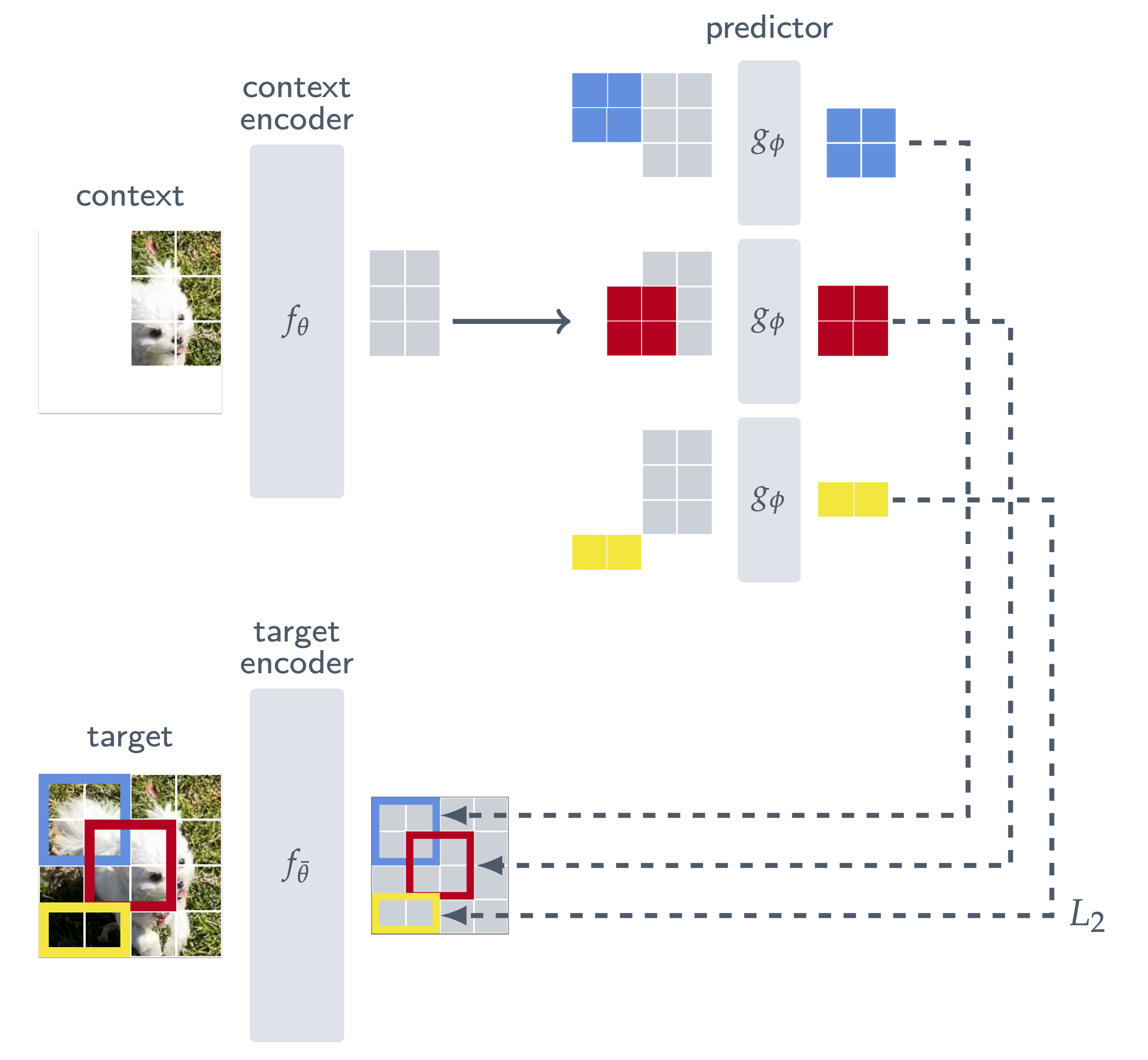
The I-JEPA architecture, conceptually close to the MAE one, begins by masking an image to define a visible context and several target regions that the model must reason about. Then, it builds on a vision transformer setup (which, remember, operates on a grid of patches) composed of three key components:
Context encoder. This encoder processes the context portion of the input image, where only a subset of patches is visible. Its goal is to get the best possible understanding of the image from this limited information, similar to the encoder in the MAE, which saw only 25% of the total patches.
Target encoder. This encoder, whose weights are an exponential moving average of the context encoder weights, processes the entire image and computes its latent patch representations. From these, only the embeddings corresponding to the target regions are selected and used as ground truth. The full image is processed before isolating target regions to ensure that the representations are fully contextualized.
Predictor. Sitting on top of the context encoder, this module learns to predict the target embeddings based solely on the visible context embedding. In other words, it takes the encoded context representation, probes it with a target position, and asks: “What would be there if we looked?”, but in latent space terms.
So, to put it in a single sentence: the goal is to predict the target encoder’s latent representations of unseen patches, prompting using only the representation of the visible context and their position.
To give a practical example, imagine showing the model part of an image that contains the body of a goose with white feathers and a long neck. Based on this visible context, the model is asked to predict what is in a masked region where the head or the legs would typically be. Crucially, the goal is not to generate the exact pixels of these but to predict the abstract embeddings that represent those concepts.
Now, how do we form the context and the target regions? And how do we tell the predictor where to predict?
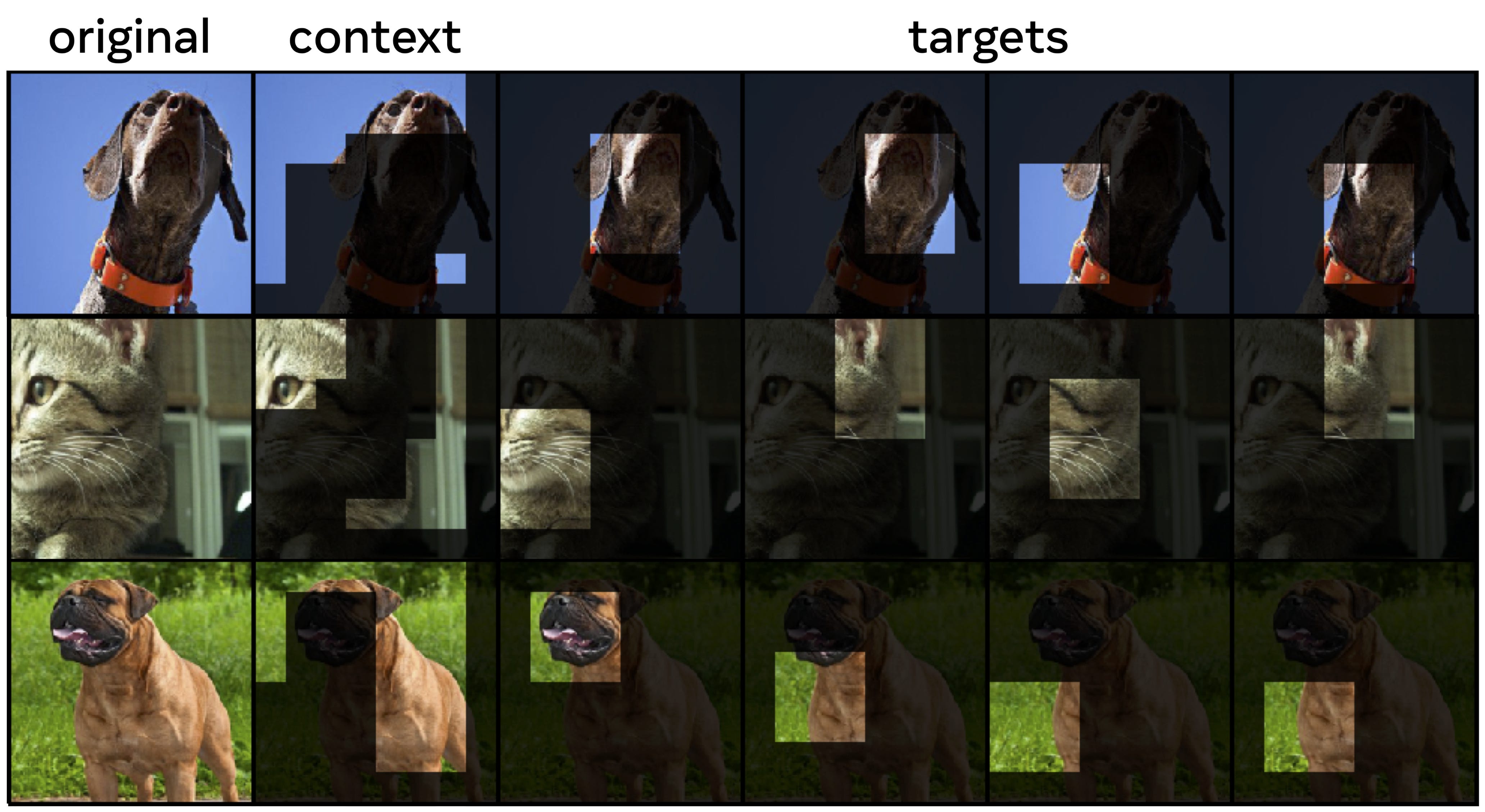
As for the target, we first divide the full image into non-overlapping patches and feed them through the target encoder to obtain patch-level representations. This results in a grid of latent feature embeddings, one per patch. From this grid, we sample four groups with possible overlap covering about 15–20% of the image area each. Note that the target blocks are obtained by masking the output of the target encoder, not the input.
As for the context, we begin by sampling a single large square block from the image, covering 85–100% of its area. To avoid leakage and ensure a meaningful prediction task, we remove any regions that overlap with the targets from this context crop. Note that this masking occurs in input space, and it is feasible because of the correspondence between the input grid and the feature grid.
As for the predictor, recall that the goal behind I-JEPA is to predict the target block representations from a single context block. This network takes the context embedding and a mask token for each patch we wish to predict with positional embeddings (colored in the figure above). Sounds familiar? Yes, it’s the MAE design again. Since we wish to make predictions for four target blocks, we apply our predictor four times, each time conditioning on different positions.
And that’s pretty much it! I-JEPA essentially reuses the logic of MAE in the encoder that processes only visible patches and the predictor that takes context and positional embeddings. However, unlike MAE, the square loss is computed not on raw pixels but on latent features produced by the target encoder. At the end of training, we take the context encoder as the backbone to produce meaningful downstream embeddings.
Performance
I-JEPA sounds very elegant, but is it also effective in practice? Well, when pre-trained on ImageNet without labels and then probed or fine-tuned using just 1% of the labels, it outperforms prior single-view methods like MAE despite being trained for 5× fewer iterations. It also matches the performance of view-invariant approaches like DINO and BYOL (not shown here), and surpasses them with the largest variant, showing strong scaling behavior.
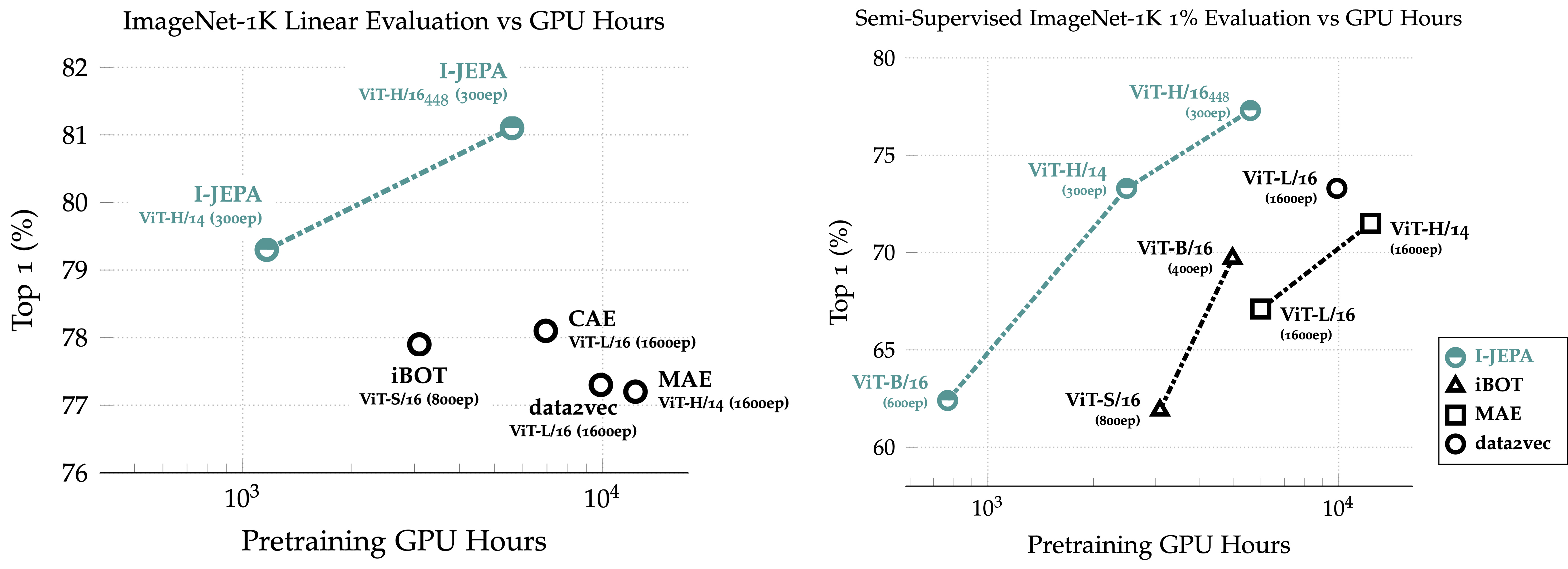
Sadly, though, the largest model is only pretrained on 15M images. Because of that, in practice, I personally still found I-JEPA to underperform compared to expectations. Reason is that the scale and diversity of the data in CLIP or DINOv2 [2], compared to ImageNet-1k or ImageNet-22k, is just unmatched in terms of producing more robust and transferable representations for downstream production use cases.
That said, there’s nothing to take away from what I-JEPA accomplishes, and we’ll see further down the line how this approach also extends to video in great fashion!
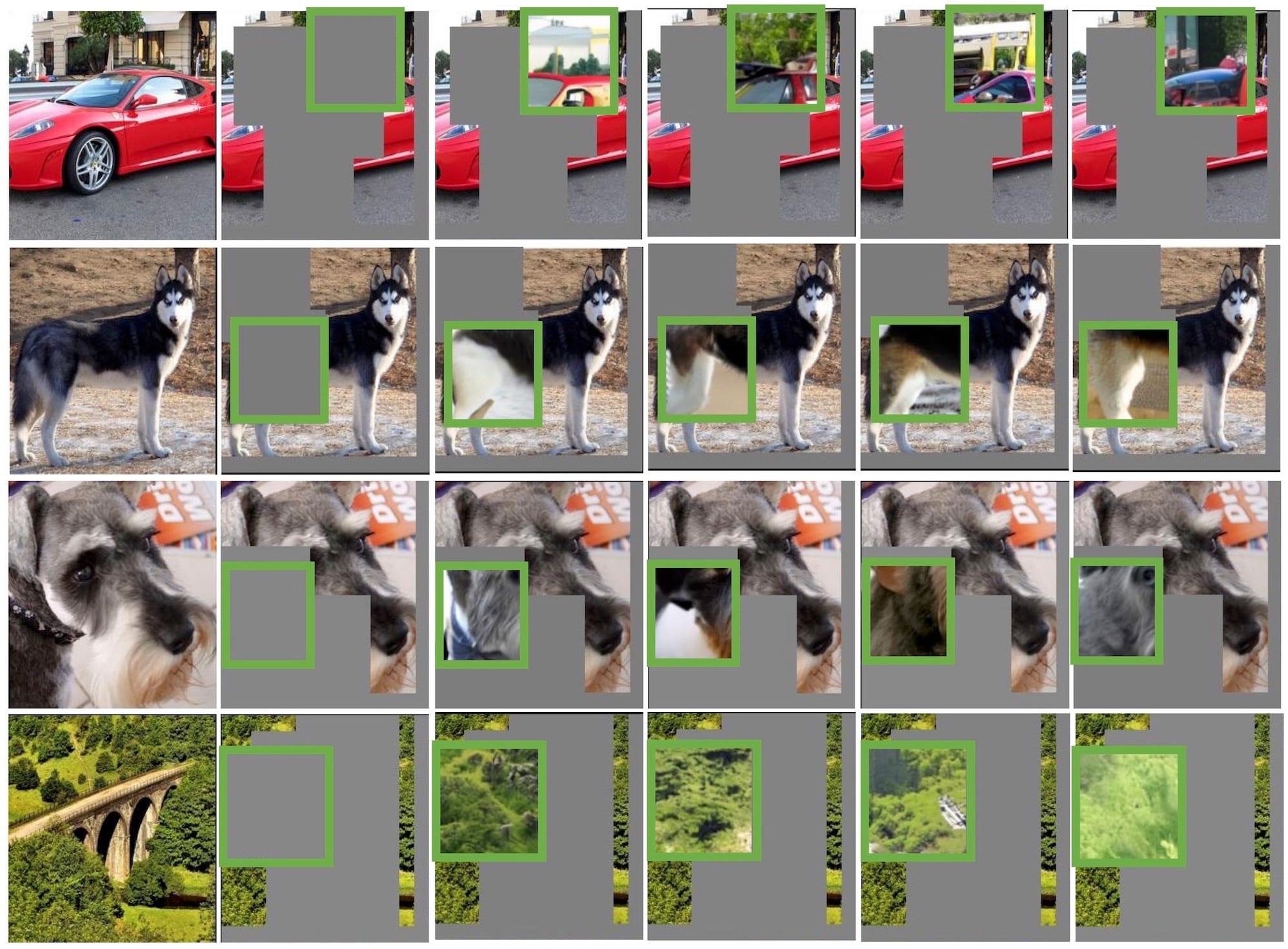
Visualizing the predictor
The predictor takes the output of the context encoder and, conditioned on positional mask tokens, predicts the representations of a target block at the specified location. Does the model correctly capture the pixel uncertainty at the target location?
To qualitatively investigate this, the authors train a generative model that maps the average-pooled predictor outputs back to pixel space. This allows visual inspection of what the model believes is likely to be in the given masked region, and also reveals whether it encodes a low-variance guess or maintains a distribution of multiple plausible completions. At the end of the day, there is not a single correct answer most of the time, and that was a big limitation in MAE.
As we can see below, the I-JEPA predictor correctly keeps some level of positional uncertainty and produces high-level object parts with the correct pose. This is a sign that the compressed latent space allocates its capacity to essential semantic cues rather than low-level details like specific colors.
Conclusions
We have seen I-JEPA, a new SSL paradigm focused on predicting representations rather than raw pixels. That alone may sound like a subtle change from MAEs, but it unlocks several benefits, including faster convergence, better abstraction of high-level semantics, and greater robustness to noise.
This learning in latent space is deeply inspired by what Yann LeCun has advocated for years: models should predict the world in abstract, compressed forms, like our brain does, not in raw sensory detail. We as humans don’t memorize pixels but learn abstract concepts from context, and this class of algorithms tries to mimic that.
Unlike MAE, I-JEPA brings back strong linear probing performance and does not require full fine-tuning to unlock useful representations. But yeah, for your image retrieval or embedding tasks, probably still better to stick with CLIP or DINOv2 for now. Thanks for reading this far, and see you in the next one!
References
[1] Self-Supervised Learning from Images with a Joint-Embedding Predictive Architecture
[2] DINOv2: Learning Robust Visual Features without Supervision