
33. Visual Anagrams
Generating multi-view optical illusions with diffusion models

Introduction
Great optical illusions are one of those things that leave everyone stunned, both young and old. They are playgrounds for artists, puzzles for neuroscientists, and a surprisingly interesting area of research in computer vision.
Today, we take a look at Visual Anagrams [1], a really fun paper that generates visual illusions using diffusion models, so that the created images transform into entirely different scenes when flipped, rotated, or rearranged as a jigsaw puzzle.
All of this happens at inference time, requires no model fine-tuning, and is just about a clever manipulation of noise. And behind the cool visuals lies a useful lesson about symmetry, structure, and the behavior of generative models, so let’s go through it!
The model behind it: DeepFloyd IF
The images in Visual Anagrams are generated using DeepFloyd IF, a high-quality 1024×1024 diffusion model developed by Stability AI, the same guys behind our beloved Stable Diffusion.
The key peculiarity of this model is that it operates directly in pixel space, unlike the more common latent diffusion models we discussed before, which generate images in a compressed latent representation and decode them afterwards using a VAE. This design is pretty much the same used in the first version of Imagen by Google [2].
Pixel diffusion is notoriously computationally expensive, so why do it? According to the paper, working in pixel space helps avoid certain types of artifacts that often show up in latent diffusion and that could easily break the illusion. As for the model, well, it technically does something a bit smarter. DeepFloyd IF uses a three-stage cascaded pipeline, conditioned on the text prompt at all stages:
It starts by generating a 64×64 low-resolution image in pixel space
This gets upsampled to 256×256, using an upsampling U-Net
Finally, another super-resolution U-Net scales it to the final 1024×1024 output.
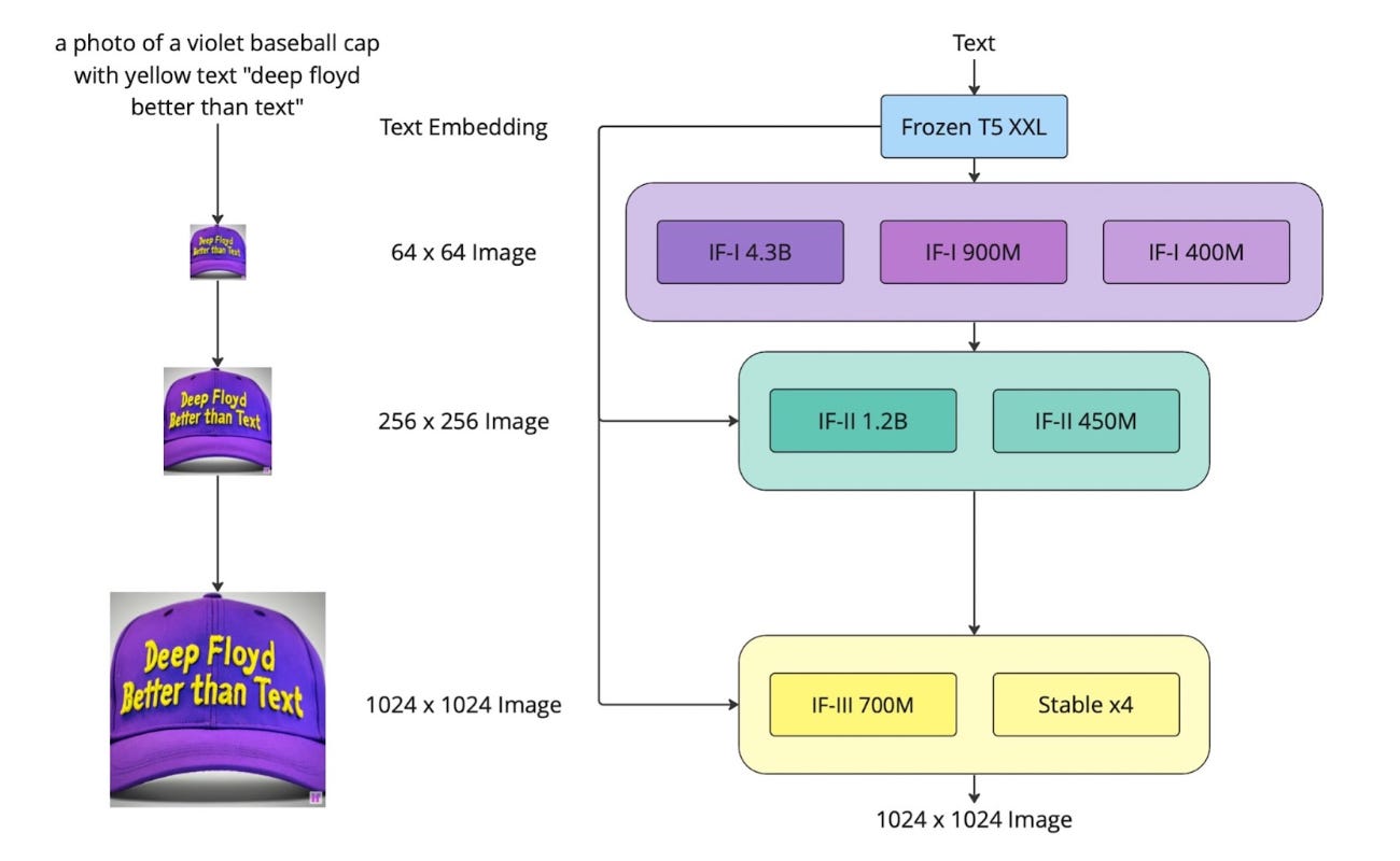
In Visual Anagrams, only the first two stages are used to craft the multi-view illusion at 256×256 resolution. The final upsampling to 1024×1024 is done using an external 4× upscaler, due to the third-stage model never being released. Anyway, now that it is clear that in this case we work in pixel space, let’s see how the illusions are created.
Method
As should be well known by now, diffusion models gradually transform pure noise into an image through a series of denoising iterations. At each step, following a predefined schedule, they predict and subtract a portion of the noise, eventually revealing a clean image in the case of text-to-image generation.
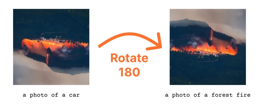
Now, suppose you want to generate a particular image that looks like:
“Prompt A” when viewed normally, and
“Prompt B” when transformed via a function T, such as a 180° rotation.
Here’s an example, where the image is both an old car and a wildfire. Pretty cool, no?
Now, as you might have guessed, we need to keep things under control at every denoising step. Otherwise, there’s no way we could generate a car in one view and somehow end up with a forest fire in the other. The key is to sample a single image that works for both views by enforcing an agreement constraint at each step.
More specifically, at each denoising step, we take the current noisy image, pass it to the denoiser with prompt 1, and get a noise estimate ϵ1. After that, we apply the transformation (e.g., rotation) and do the same with prompt 2 to get another noise estimate ϵ2. These two predictions are then aligned by applying to ϵ2 the inverse of the transformation used to create the second view and then averaged. Using that noise to perform the denoising step ensures consistency across both views.
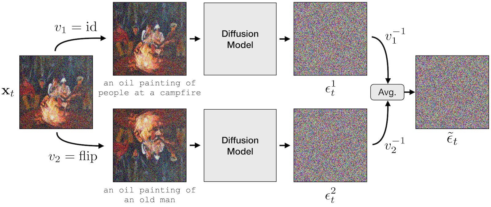
To stress that again: once we average the predicted noise, the standard denoising step is taken only in one canonical view. The model doesn’t generate or update two images separately but rather keeps the views in sync through the denoising process. This is as simple as asking the two questions at each timestep:
What noise do we need to remove to make the image look more like prompt 1?
What noise do we need to remove to make the transformed image (which is nothing but the first one flipped, rotated, or so) look more like prompt 2?
Averaging keeps both constraints satisfied at a high level, with the trade-off being a loss of some information because of the mixing. Now that we saw the fun part, time to step back and reflect on why this works. At its core, it is all about manipulating noise, but in a way that is far from straightforward.
What makes a valid transformation?
Generative models expect a certain level of noise for a given timestep t, and they are trained to remove structured noise in a way that reflects both the input and the step. That’s because, during training, the model sees inputs that have a known amount of Gaussian IID (independent and identically distributed) noise added to them and learns to reverse that process. Anything that breaks that assumption causes the model to fail, for example:
Using the wrong noise for a timestep. Asking the model to denoise a very noisy image, pretending that “we are at the end of the process”, where the expected noise level is minimal, won’t work. For each timestep, there is a specific linear combination of pure noise and pure signal that the model was trained to expect.
Using the wrong kind of noise. Even if the signal-to-noise ratio is correct for the current timestep, non-Gaussian or spatially correlated noise breaks the model expectations. Noise must be IID.
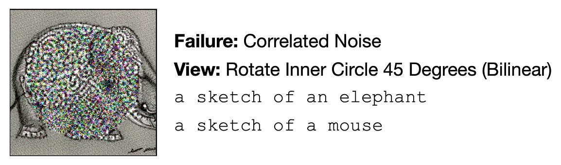
So, in order to make the illusion work, the transformed noise must also satisfy the statistical assumptions for that timestep. See a failure case below, where the illusion was to rotate a circle centered at the center by 45°. Due to bilinear interpolation of the pixels when applying the transformation, noise is no longer IID, and it stays there.
To preserve the linear combination of signal and noise, we need to apply a linear transformation A to the image. As for the statistical assumptions, we must ensure that our transformed noise Aϵ is still drawn from a standard Gaussian. This is a stricter requirement, and it holds true if and only if A is an orthogonal matrix. This comes from the spherical symmetry of the Gaussian.
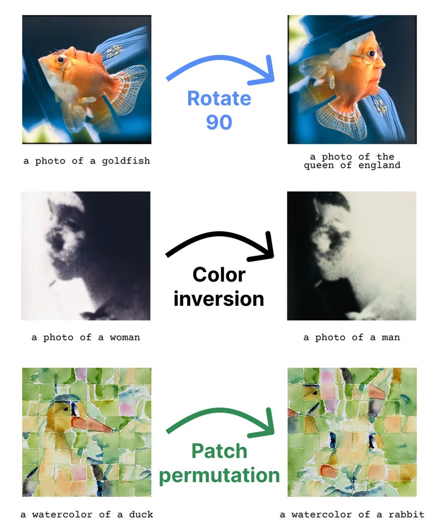
So in conclusion, the method is constrained to orthogonal transformations, which preserve pixelwise noise statistics. This still includes a wide range, such as:
Rotations (but with caution for non-multiples of 90°, due to interpolation)
Flips and spatial reflections
Color negation
Pixel and patch permutations (e.g., jigsaw)
Partial skews or region-specific transforms
Combinations of the above, e.g., even 3 or 4 rotations!
More generally, any rearrangement of pixels in an image is good, hence the name “visual anagrams”. Here are some cool examples, but for a full display, you should totally check out the project website at https://dangeng.github.io/visual_anagrams/.
Conclusions
Using diffusion models to create visual anagrams is a great reminder that we do not always need to train new models from scratch. Sometimes, all it takes is a deep understanding of how existing models operate and fantasy within their constraints.
With this work, we have seen that it is possible to squeeze fun capabilities out of diffusion models and that test-time noise manipulations can be very successful. However, breaking the modeling assumptions even slightly can lead to catastrophic results. Always make sure you understand the space in which models operate!
Personally, I am very hooked on the topic and find some beauty within these kinds of test-time prediction steering frameworks. Hope you enjoyed the bit more lightweight content at the intersection of generative modeling and art, and see you next week!
References
[1] Visual Anagrams: Generating Multi-View Optical Illusions with Diffusion Models
[2] Photorealistic Text-to-Image Diffusion Models with Deep Language Understanding
I saw your post on Linkedin and was glad to see that you had a detailed post about it! I love the posts because of your style of writing, it's clear and has voice and explains these cool concepts without resorting to AI (as so many people do, unfortunately!). Will stay tuned :))