
36. DIFT: DIffusion FeaTures
Extracting semantic and geometric correspondences from diffusion models

Introduction
Finding pixel-wise image correspondences is a central step for tasks such as tracking, 3D reconstruction, and image editing. Yet, building supervised models for it remains challenging, since dense annotations are costly to obtain outside of synthetic settings.
On the other hand, it is well established that powerful representations emerge from large-scale pretraining. “Emergent Correspondence from Image Diffusion” [1] proves that pixel-level correspondences naturally show up also in generative models like Stable Diffusion, even without an explicit training objective designed to encourage them!
This leads to DIffusion FeaTures (DIFT), a method to extract these pointwise matches from diffusion U-Nets. Without any fine-tuning, DIFT proves to be robust and handles semantic, geometric, and temporal correspondences with ease. Let’s go!
Method
Establishing reliable correspondences between images is typically approached with a standard pipeline consisting of two stages (plus an optional verification):
Pointwise feature extraction. First, we identify keypoints or interest points in the image and compute feature descriptors that represent the local context around them. This can be achieved with hand-crafted methods, such as SIFT [2], or with learned approaches like SuperPoint [3], which adapt features directly from data.
Feature matching. Second, these descriptors are compared across different images to identify the most likely matches. Simple approaches rely on nearest-neighbor search in descriptor space, while more recent methods use models that predict correspondences directly.
(Optional) Verification. Especially in the case of geometric correspondence, incorrect matches from stage two can be filtered out by enforcing consistency with a global constraint (e.g., camera pose change). However, this stage cannot be applied in the case of semantic correspondences, which are way more abstract.
In the case of DIFT, we operate somewhere between stage one and stage two. Instead of explicitly designing descriptors (stage one) or training a dedicated matching model (stage two), DIFT takes keypoint locations as input and retrieves features representing them from the forward pass of a diffusion U-Net. Then, it matches features across images by simple nearest-neighbor search, delivering correspondences.
More in detail, here are the key steps to get DIFT:
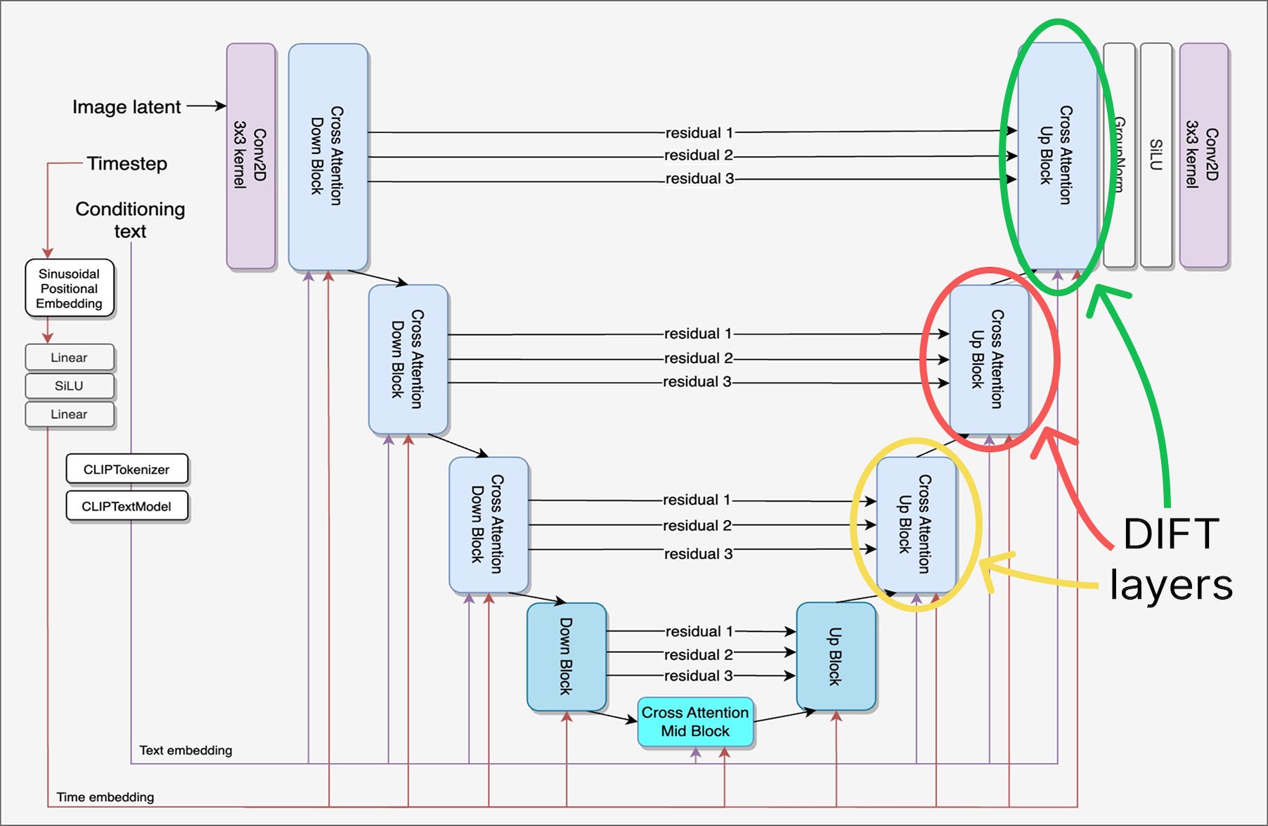
Encode the input image into latents using the VAE encoder, since SD is a latent diffusion model and the denoising U-Net never sees pixels.
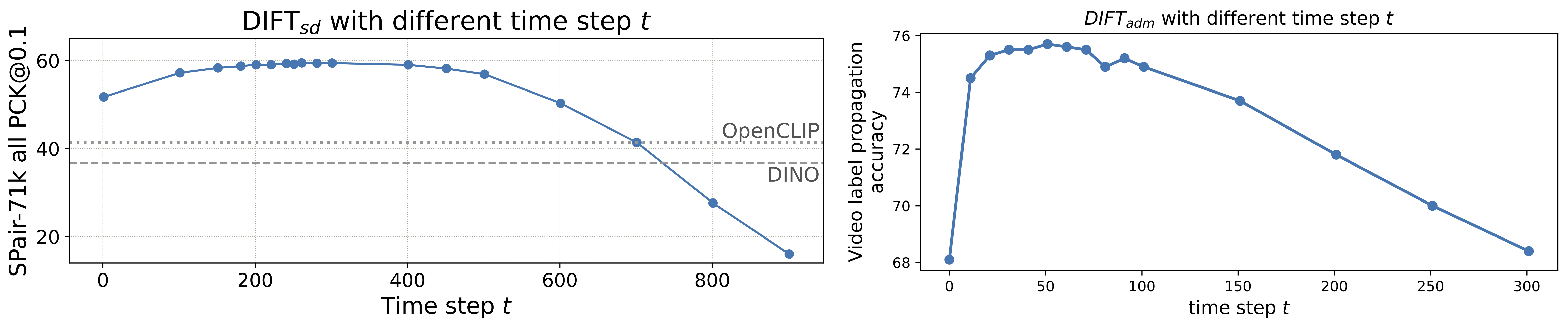
Add diffusion noise at a chosen timestep t to simulate the forward diffusion process. A timestep more toward the end works best, as the noise level is not so high. More on that later, but semantic tasks benefit from a slightly larger t, while geometric tasks use a smaller t.
Feed the noisy latent to the diffusion U-Net, along with its t, and a simple prompt describing the original content (or even the empty string).
Extract an intermediate layer’s features from the up blocks of the U-Net. These are the DIFT descriptors, which have an image-like structure but with C channels instead of the three in RGB, where C depends on the layer selected. In essence, they are standard feature maps at a lower spatial resolution. Given any position p on this latent grid, one can interpolate and have a descriptor F(p) of dimension C.

Different feature extraction possibilities in the up block of the diffusion U-Net. Image from https://arxiv.org/pdf/2306.09762 Match features between images via nearest neighbor using cosine distance. Since positions in the latent grid relate to locations in the original pixel space, we can compare descriptors across images for any pixel location p in the first image by looking at its latent grid F1. Concretely, we take the feature grid F2 from a second image, and find the position q that minimizes the distance between F1(p) and F2(q). We call these two points p and q a correspondence.
More generally, this nearest-neighbor matching can be applied to other vision backbones. It works particularly well with vision transformers, since they strictly preserve the spatial layout of image patches as information flows through the layers. Highly semantic backbones like CLIP and DINO are also put to the test in the paper.
Applications
Now that we have seen how to match pixels across images using DIFT descriptors, we can outline some of the main applications that become possible when you have this dense, geometry-aware correspondence:
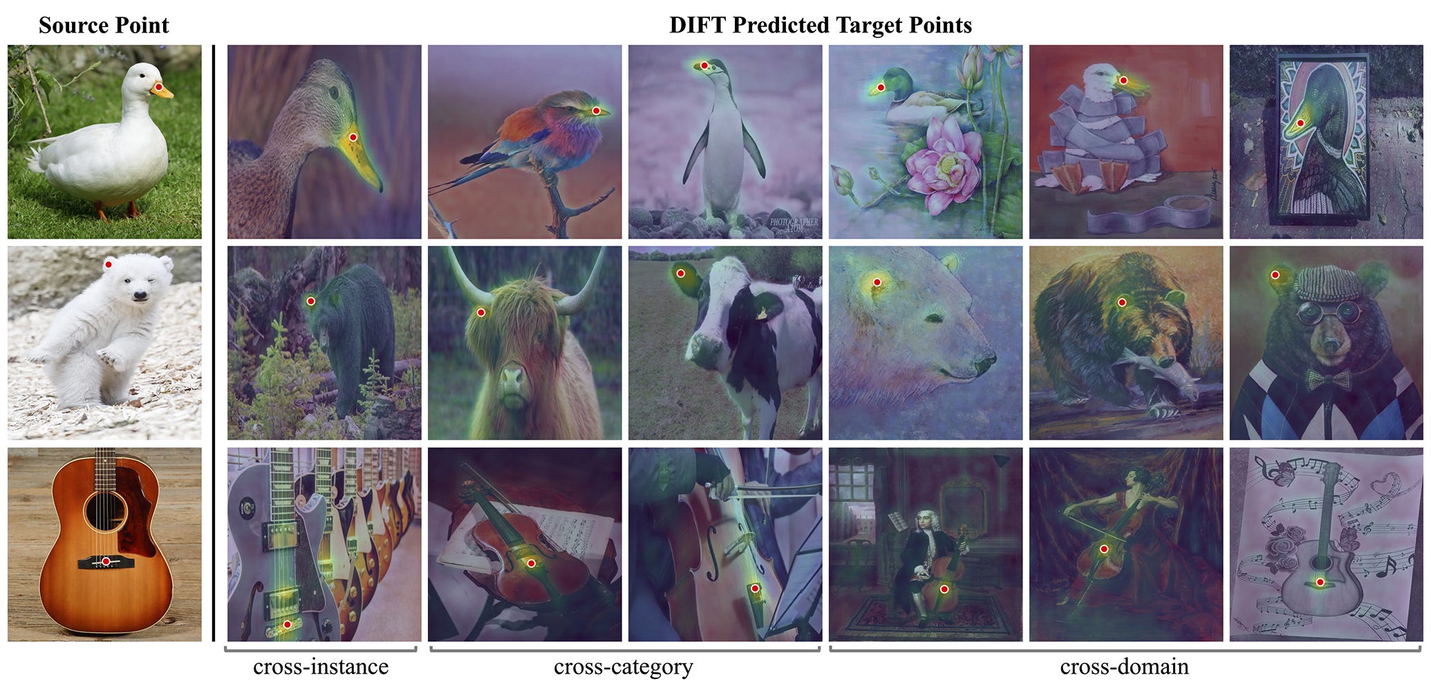
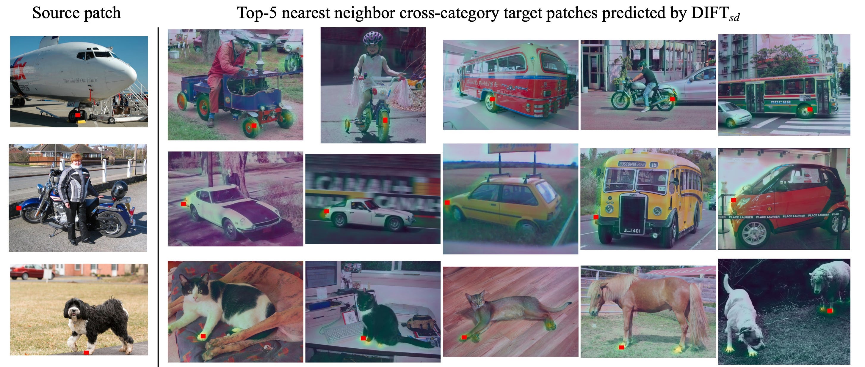
Semantic correspondence, i.e., looking for pixels of different objects/animals that share similar semantic meanings. For example, matching the beak of a goose to the beak of an eagle, even across different objects or species.
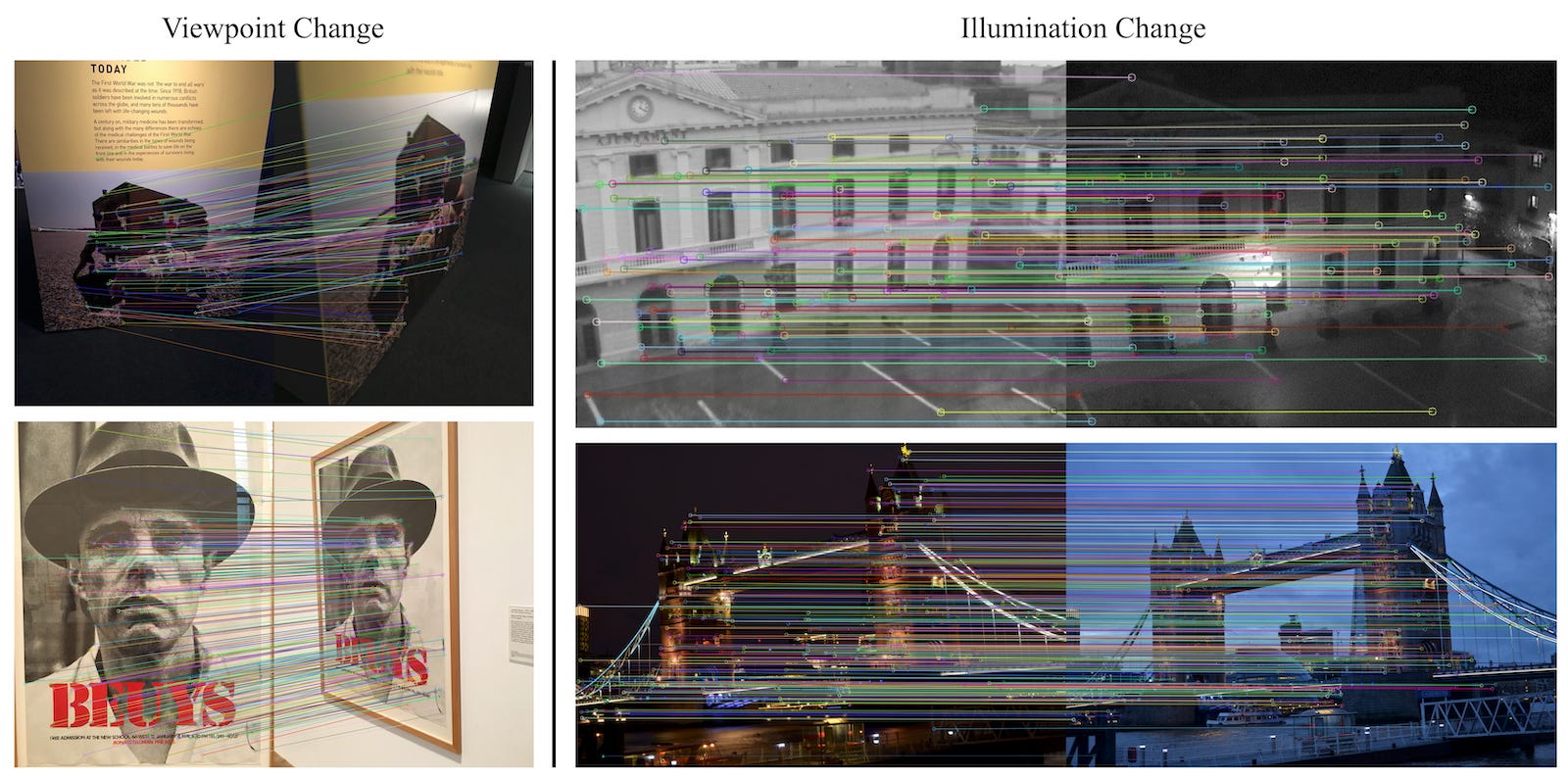
Geometric correspondence. This task is about finding pixels of the same object captured from different viewpoints. It is particularly useful in 3D reconstruction pipelines to estimate camera poses and triangulate points.
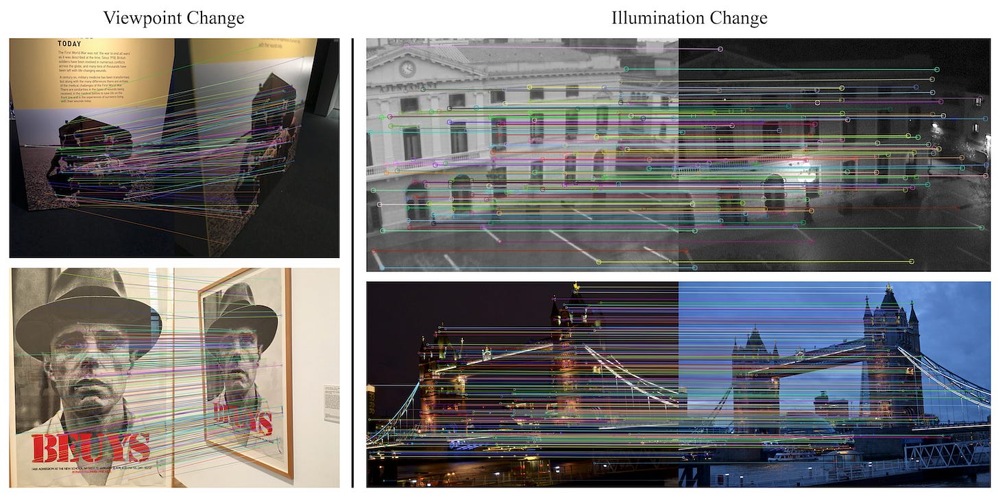
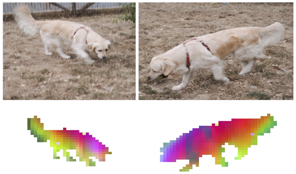
Example of sparse feature matching using DIFT for geometric correspondences. Image from [1]. Temporal correspondence. Finding pixels that refer to the same point across time in a video. This is useful for object tracking and optical flow–like motion estimation.
Now, in order to run the U-Net, we need to add a certain level of noise to the encoded image latent, to simulate the reverse process of image generation that the model was trained on. Different tasks require different levels of noise, although we always use mid-to-late timesteps, of course.
In particular, semantic correspondence across different subjects benefits from more noise because this forces the model to rely on global semantics rather than low-level details. On the other side, geometric and temporal correspondence tasks typically require smaller timesteps with less noise to preserve the fine-grained spatial details needed for accurate matching.
But how robust is the method? In terms of timestep, DIFT performance is fairly stable across a wide, flat range of timesteps. The authors pick t=101 or t=261 for semantic tasks, and t=41 or t=0 for geometric ones, depending on the model used.
A second trick to make it more stable is to actually use ensembling! Instead of adding noise once and extracting features, we can add noise multiple times at the same timestep with different random seeds, run the U-Net forward in a batch, and then average the resulting feature maps to form the final representation. This is the advantage of working with generative models!
Conclusions
Once again, large pre-trained models exhibit emergent capabilities far beyond their original training objectives. DIFT taps into the denoising U-Net of diffusion models and shows that there is a strong correlation between restoring image details and understanding what is being restored.
Most importantly, this feature-matching system requires no additional supervision and showed stronger results than pre-trained vision backbones like CLIP and DINO at the time. Now, this is by far no longer true, since the pace of progress is relentless. Plain DINOv3 patches are probably crushing these old benchmarks of mid-2023.
But either way, it’s always fun to see that a model trained purely for generation can turn out to be an excellent discriminator as well. I guess the closing remark is: never try to reinvent the wheel, unless you’ve tried it all. See you next time!
References
[1] Emergent Correspondence from Image Diffusion
[2] Distinctive Image Features from Scale-Invariant Keypoints
[3] SuperPoint: Self-Supervised Interest Point Detection and Description