
43. ConvNeXt
A modern convolutional neural network for the 2020s


Introduction
For nearly a decade, convolutional neural networks were the undisputed pillar of computer vision. Although they were originally designed at the end of the last century, they truly took off in 2012 with AlexNet, followed by VGG a few years later and ResNet in 2016, with each generation becoming deeper, wider, and more powerful.
CNNs powered most of the breakthroughs in image and video understanding up to around 2021, driving progress across tasks like classification, detection, and segmentation. But eventually, their convolutional inductive biases, which had served so well for so long, started to show their limits.
As the Vision Transformer [2] arrived in late 2020, it challenged everything we thought we knew about how to process images. In a short amount of time, ViTs quickly surpassed ConvNets on benchmarks, and soon, every new model was transformer-based. But this radical shift obviously raised a question: were CNNs truly obsolete, or simply not updated in a long time?
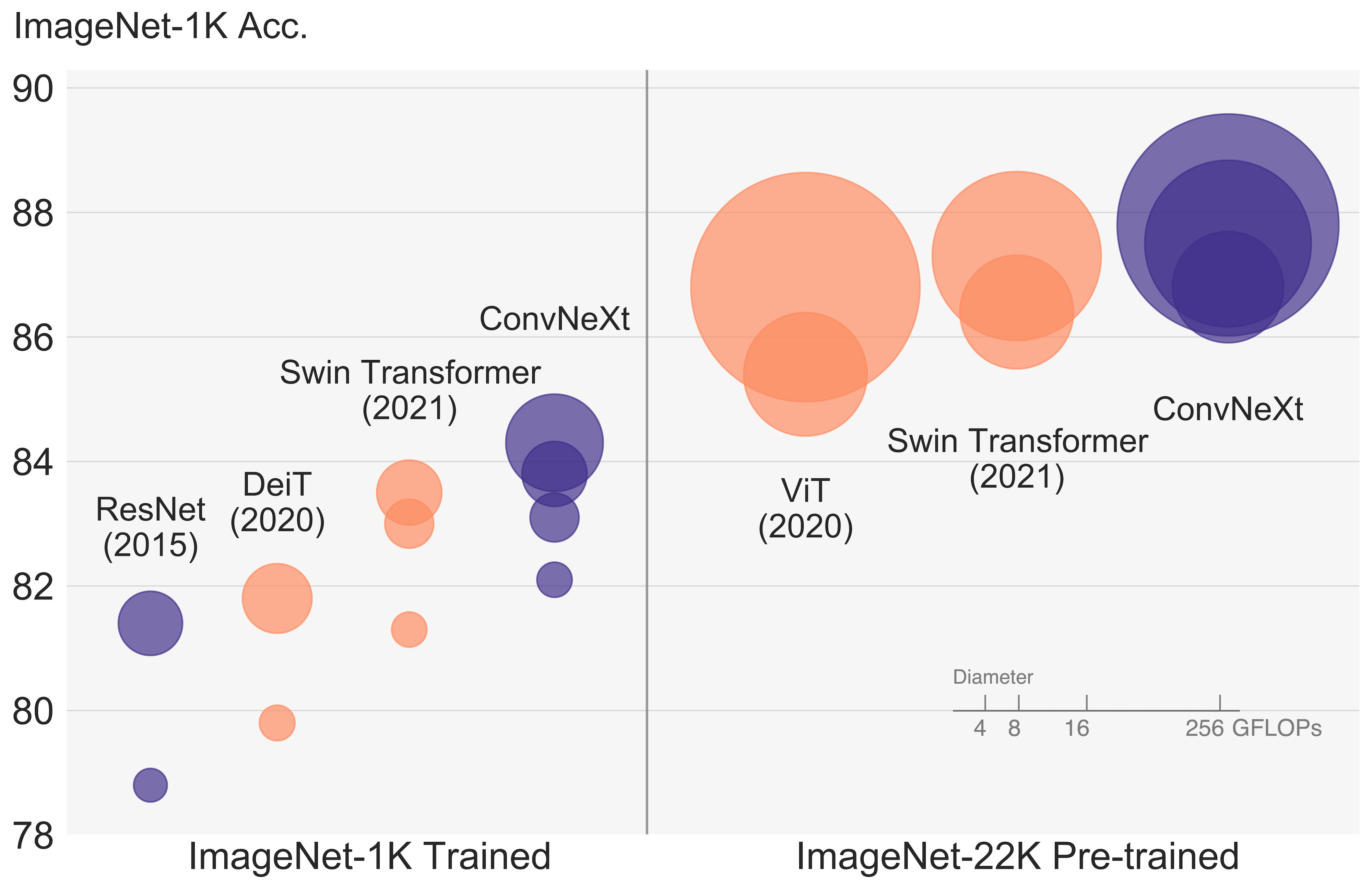
In “A ConvNet for the 2020s” [1], researchers at Meta argue that the performance gap isn’t as large as it seems once we modernize the classic ResNet [3] with a decade of learning. The result is ConvNeXt, capable of matching and even surpassing state-of-the-art transformers (in 2022) while remaining computationally efficient. Let’s take a closer look at what goes into making an old model great again!
Note: I will take for granted a basic understanding of convolutional operations. You can learn more here in case this sounds unfamiliar.
Modernizing a ConvNet
The authors started this experiment with something familiar and very strong: a ResNet-50 backbone. This is one of the most widely used convolutional neural networks in history and the one that popularized the idea of residual connections, a concept now everywhere from Transformers to diffusion models.
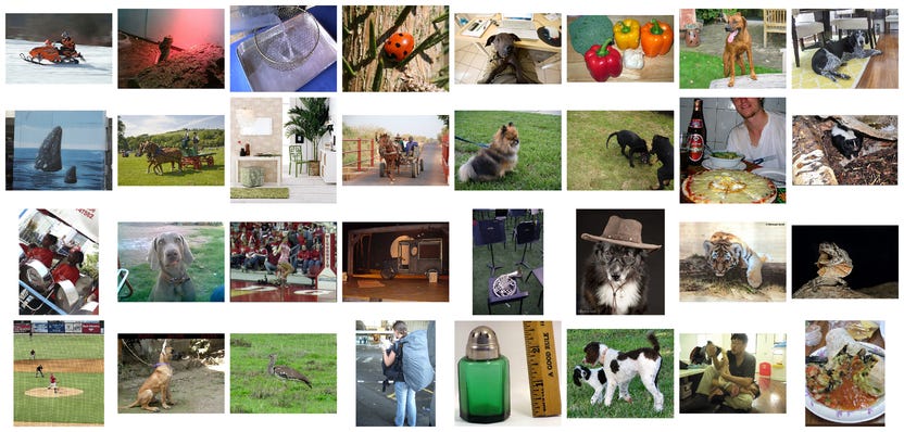
The benchmark is the ImageNet-1K dataset, and all models are trained and evaluated on it. As a quick refresher, ImageNet-1K involves classifying images into 1000 classes, ranging from animals to everyday objects, using around 1.2 million training images.
Since the search space for CNN architectures is enormous, the paper adopts a simple yet principled approach: apply one modification at a time and measure how each change affects overall performance in terms of accuracy, efficiency, and training stability. Following a clear roadmap, the idea was not to invent new tricks, but to refine what already works. Here are the six steps they took.
1. Start from ResNet, but trained in the modern way
The original ResNet-50 was trained with plain SGD and very simple augmentations such as cropping, horizontal flips, and color distortions. ConvNeXt first establishes a proper modern baseline by retraining ResNet-50 with a training recipe inspired by modern transformer practices. This includes:
Using the more powerful AdamW optimizer
Training longer, up to 3× more epochs
Cosine learning rate decay with warmup
Larger batch size (4096 vs. the original 256)
Data augmentation techniques such as MixUp, CutMix, and RandAugment
Regularization methods, including layer dropout and label smoothing.
By itself, this enhanced training recipe increased the performance of the ResNet-50 model on the ImageNet test set from 76.1% to 78.8%, without changing a single layer. This is a strong reminder that training matters as much as architecture, and recipes improve constantly over time.
2. Macro design
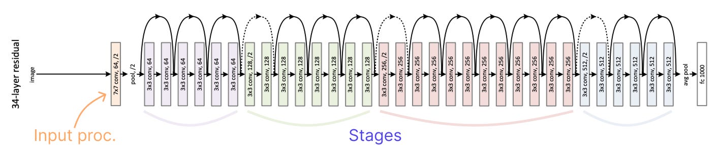
ResNet is divided into four stages, each made up of several residual blocks that operate on feature maps of the same spatial resolution. The resolution decreases only when transitioning from one stage to the next, typically by a factor of two through a stride-2 convolution.
As a first step, the authors adjusted how much computation happens in each stage, or in other words, how many blocks are allocated to each resolution level. In the original ResNet-50, these stages contain (3, 4, 6, 3) identical blocks, with most of the computation concentrated in the third stage. This design was originally conceived to support downstream tasks like object detection, where a detector head would operate at the 14×14 feature map level of that third stage.
Following the more recent design of the Swin Transformer [4], a variant of ViT used for detection and segmentation, these ratios are adjusted to (3, 3, 9, 3) blocks. FLOPs go up a bit due to adding more blocks overall, but so does performance.
As a second step, the input image processing (the orange operation) is redesigned. ResNet uses an aggressive 7×7 convolution with a stride of 2, followed by a max pool, which results in a 4× downsampling in the image resolution before entering any block. ViTs handle this differently, splitting the image into non-overlapping patches, equivalent to applying a large convolution (e.g., 14×14 or 16×16 kernel) with a stride equal to the kernel size.
To mimic this behavior, the image processing is replaced with a patchify layer similar to ViT, implemented as a non-overlapping 4×4 convolution with a stride of 4. This makes the first layer more local, capturing finer spatial details, and more efficient.
Combining these two macro changes, performance improves from 78.8% to 79.5%.
3. Depthwise and 1×1 convolutions
In a standard ResNet block, the main 3×3 convolutions mix both spatial and channel information at once. This coupling is powerful but also expensive, and that’s why ConvNeXt adopts depthwise convolutions instead.
In this variant, each channel of the feature map is processed separately, learning its own independent spatial patterns. It’s a much cheaper operation, popularized in MobileNet [5], a lightweight CNN designed for efficient inference on mobile and embedded devices.
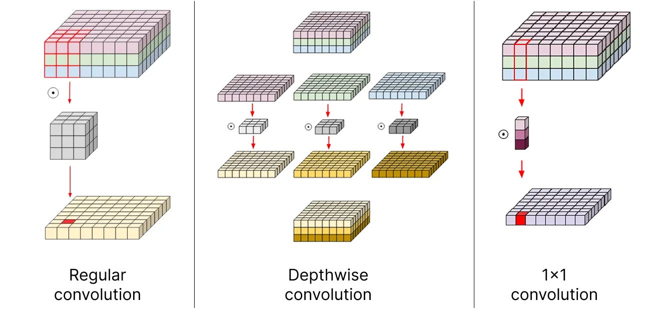
To mix information across channels, 1×1 convolutions are added. This type of operation keeps the spatial resolution the same while combining information from different channels. Simply put, each output channel becomes a weighted sum of all input channels, aka, it is exactly an MLP!
The combination of depthwise conv and 1×1 convs leads to a separation of spatial and channel mixing, a property shared by Vision Transformers, where each operation either mixes information across spatial (self-attention) or channel dimension (MLP), but never both.
This filter redesign boosts performance by another full point, reaching 80.5%.
4. Inverted bottleneck
In the MLPs, Transformers expand the feature dimension typically by 4 times in the hidden dimension before compressing it back. This expansion accounts for most of the parameters but is considered the main place where the model stores its knowledge.
Within each block, ConvNeXt momentarily adopts the same inverted bottleneck structure (b), first using the 1×1 convolutions to perform the change in dimensions (e.g., 96 to 384 channels), and then doing the 3×3 depthwise convolutions at the expanded dimension.
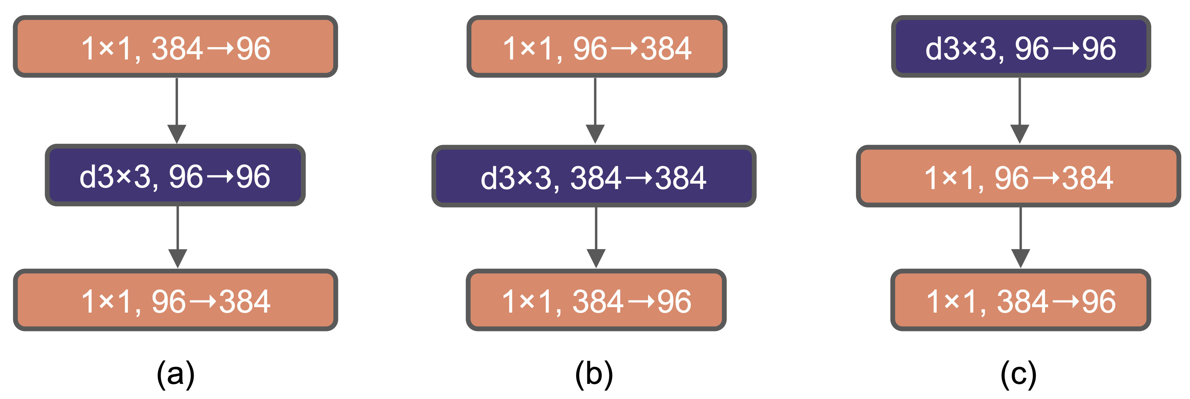
These changes practically leave performance invariant (+0.1%) but make the model more efficient than (a), thanks to the significant reduction in FLOPs that occurs between stages, where the convolution layers with stride 2 used for downsampling now operate on fewer channels.
5. Large kernels
Traditional ConvNets use 3×3 filters, which have efficient hardware implementations on modern GPUs. Stacking several 3×3 layers allows information to slowly flow across a wider spatial area without a large computational cost. On the other side, ViTs have a global receptive field from the start, thanks to the self-attention mechanism.
To achieve a similar improved receptive field, significantly larger kernel sizes must be used in ConvNeXt. To explore these, one prerequisite is to move the position of the depthwise conv layer up, i.e., adopting configuration (c) as final. This new design places the less efficient operations where there are fewer channels, while the efficient, dense 1×1 layers do the heavy lifting, making the use of large kernels actually feasible.
After this adjustment, the kernel size can be increased from 3×3 to 7×7 in the depthwise convolutions. Larger sizes experimentally do not provide any additional benefit. With this change, the performance reaches 80.6%. It’s again a small improvement (+0.1%) compared to before, but in practice, larger kernels completely redesign the dynamics of the network.
6. Micro design adjustments
After all the previous global-scale changes are implemented, and the CNN starts gaining performance in part by borrowing ideas from the ViT architecture, a few layer-level details are further proposed to squeeze out more juice. In particular:
The ReLU activation function is replaced with the smoother GELU activation, used in a lot of frontier LLMs at the time. Activation functions are continuously questioned today, as they can make a noticeable difference at large pretraining scales, and this is actually already outdated!
Inspired by the design of transformers, the number of activation functions is reduced from one after each convolutional layer to just one per block, simplifying the computation and surprisingly making the model more performant (+0.7%)
Similarly, fewer normalization functions are used, mimicking the single normalization before each transformer subblock, and BatchNorm is replaced with LayerNorm used in transformers, improving training stability (+0.2%)
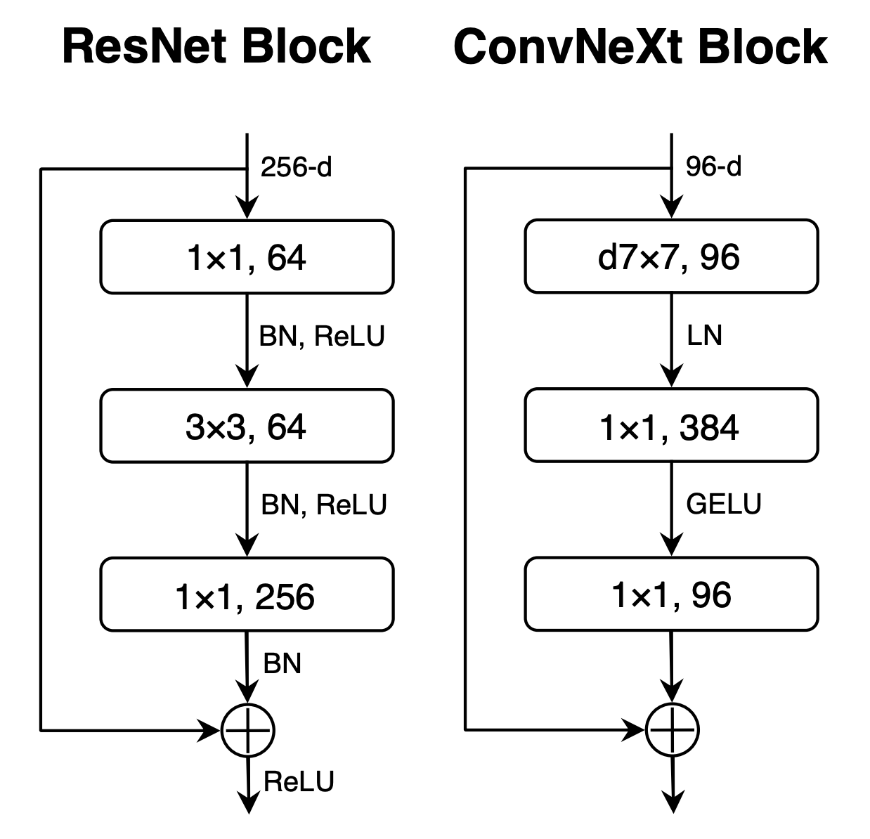
Final block design for ResNet and ConvNeXt. Note that there are many fewer activations and normalizations, as well as a larger kernel. Finally, downsampling layers between stages are implemented as 2×2 convolutions with stride 2 instead of the overlapping 3×3 convolutions used in the original ResNet. To stabilize training, additional LayerNorm layers are introduced around those resolution changes, and this boosts the final accuracy to 82% (+0.7%), significantly exceeding the ViT baseline.

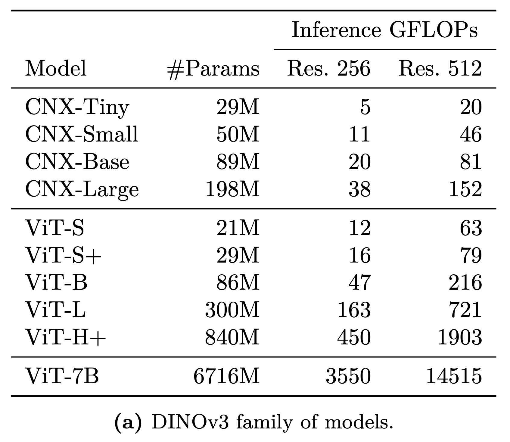
With these refinements, the ConvNeXt architecture emerged. It is modern, efficient, and powerful, combining the strengths of convolutional networks with the design principles of transformers. However, you might ask: why use a CNN when transformers exist? The answer lies in FLOPs! ConvNeXt models allow inference with larger architectures or higher image resolutions than ViT for a fixed computational budget, offering a better frontier between performance and efficiency. See the table below to get an idea:
Conclusion
We saw ConvNeXt, a modern CNN that renovates the iconic ResNet by integrating a decade of architectural and training improvements, along with the design principles of the ViT architecture. Thanks to these updates, the ImageNet accuracy jumps from 78.8% to 82.0%, establishing a new state of the art for convolutional networks and showing that with brilliant modernization, efficient classic architectures can still compete at the highest level.
ConvNeXt comes in several variants (T, S, B, L, and XL), ranging from about 29M parameters up to 350M for the largest model. Today, this architecture is stronger than ever, as for all but the XL variant, DINOv3 [6] distills the features of the largest 7B-parameter ViT into it. It goes without saying that combining the best model with the best data makes it pretty hard to beat, making DINO-ConvNeXt arguably the best CNN checkpoint to start from for your experiments on custom domains.
Thanks for your attention, and see you soon! I’m trying to get back to a weekly posting schedule, but things are still quite busy around here, and I don’t want to overpromise. In any case, thank you so much for your support and for helping the blog pass 1000 subscribers: it’s incredibly motivating and means a lot!
References
[2] An Image is Worth 16x16 Words: Transformers for Image Recognition at Scale
[3] Deep Residual Learning for Image Recognition
[4] Swin Transformer: Hierarchical Vision Transformer using Shifted Windows
[5] MobileNets: Efficient Convolutional Neural Networks for Mobile Vision Applications
[6] DINOv3