
47. DiT: Diffusion Transformer
Understanding the architecture behind Stable Diffusion 3, FLUX, and Sora

Introduction
Image generation was originally synonymous with U-Nets and their characteristic downsampling and upsampling blocks. In fact, they were chosen as the default backbone for denoising diffusion when DDPMs first arrived, survived the shift to latent space, and finally became mainstream with Stable Diffusion (if you need a recap, all of these are covered in posts #8, #16, and #17).
Adopting this architecture made sense because denoising requires predicting a tensor of the same dimensionality as the input. It also needs a constant reference back to the input to refine the prediction, which is handled effectively via skip connections. On top of this, the U-Net architecture was already proven successful for dense tasks like image segmentation, and predicting the noise added to each pixel or latent code is, at the end of the day, just another dense task.
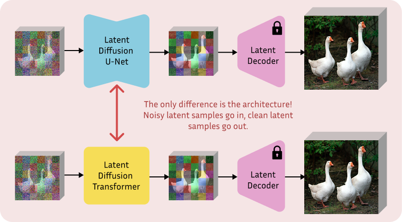
But in late 2022, the community genuinely asked: what if we use a plain transformer instead? The result is a new denoiser named Diffusion Transformer (DiT) [1] and an architecture still prevalent today, powering all the state-of-the-art models in the image and video generation domain. Let’s analyze the difference.
NOTE: In this post, I refer to DiT primarily as an image denoiser. However, the architecture is modality agnostic: it applies equally to image, video, text, and audio generation.
Denoising U-Net: a hybrid backbone
The issue with a fully convolutional U-Net is not a lack of functionality, but rather that it would come with restrictive inductive biases, specifically a local receptive field. This is far from ideal for media generation, where global coherence is necessary.
For this reason, denoising U-Nets actually end up borrowing two key elements from transformers, making them some kind of hybrid models:
To compensate for the limited receptive field and capture interactions across distant input regions, they use self-attention between all spatial positions.
To handle external conditioning like text prompts, they rely on cross-attention. Here, the intermediate spatial features of the image act as queries that attend to the text embeddings, serving as keys and values.
Concretely, in models like Stable Diffusion 1.x and 2.x using a latent U-Net, this happens by temporarily reshaping tensors from B×C×H×W into B×(H·W)×C. The model treats these as a standard sequence of tokens during attention computation before reshaping them back into an image-like tensor for the next convolutional block.
So when we look back, this architectural shift from U-Net to DiT actually looks less drastic. The attention mechanism powers both models at their core. With that in mind, let’s see what changes when using a regular transformer.
The DiT backbone
Simply put, the DiT architecture in the image generation domain is basically a Vision Transformer repurposed as a noise predictor: image patch tokens go in, and noise predictions for each token come out. The whole thing is reduced to minimal complexity, relying on a stack of plain transformer blocks. It is useful to have a visual summary of the full architecture here before diving deep into the components.
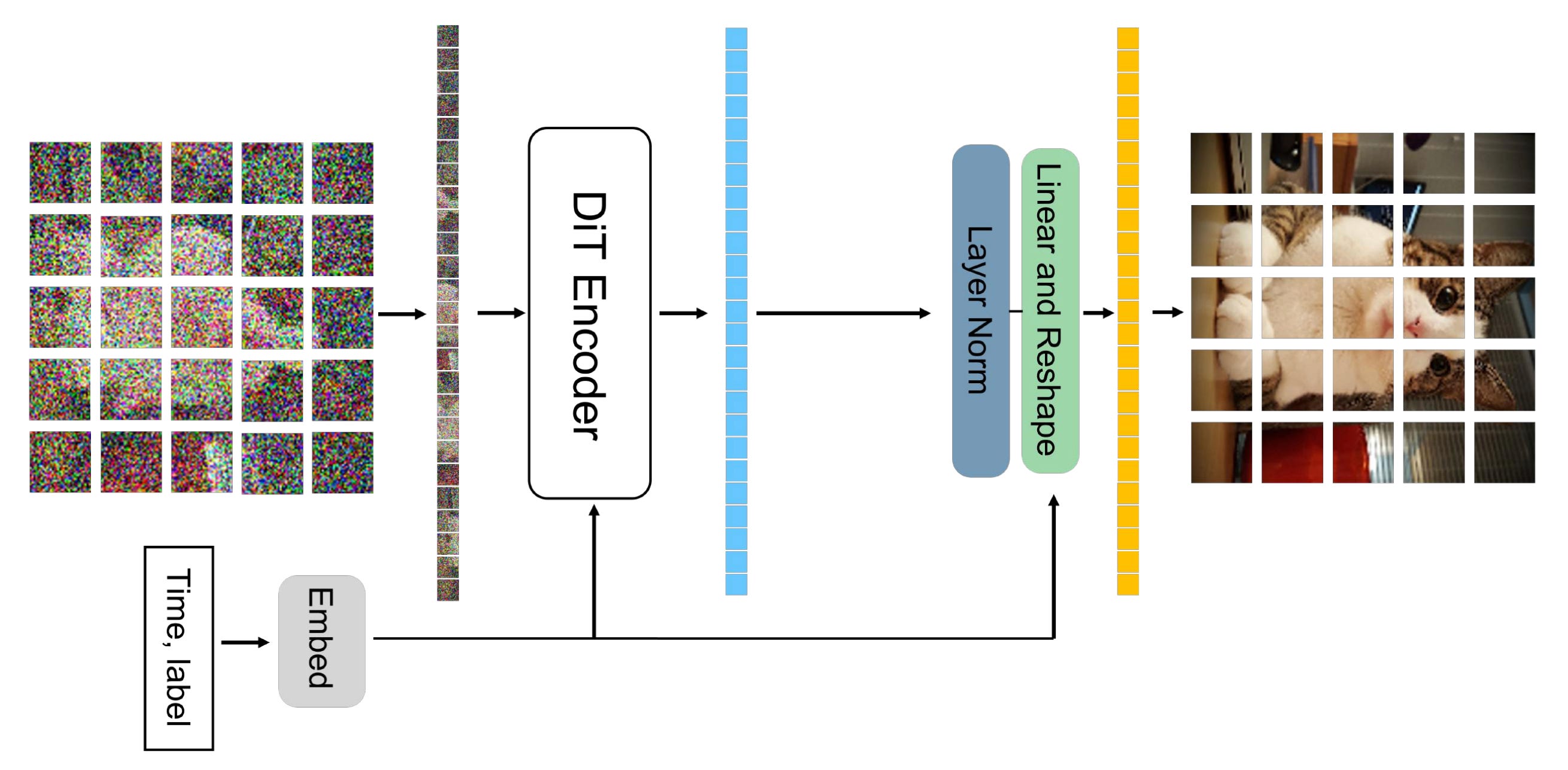
Now that we have this in mind, let’s go through the denoising process from the point of view of an image:
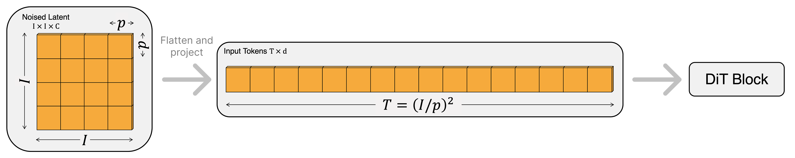
Patchify. Both at training and at generation time, the input to DiT is a noisy encoding in the latent space of a VAE. Assuming no batch dimension, this input is structurally a 3D tensor H×W×C that looks just like a small image with extra channels (C=16 is the common choice these days). The first DiT layer handles this by breaking the grid into little non-overlapping squares, exactly mirroring the patchify step of a standard ViT.
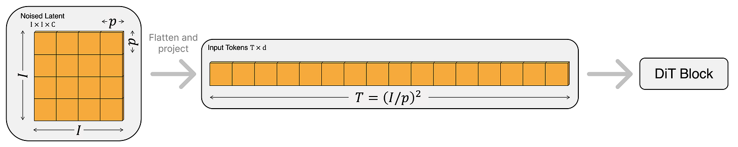
The latent, shaped like a VAE encoded image, is divided into non-overlapping patches with a small patch size (e.g., 2x2), each flattened and linearly projected into a token embedding. From [1]. For example, if we use a patch size of 2, the model groups every 2×2 window of “latent pixels” into a single block. Continuing the example with 16 channels per pixel, one patch would contain 2×2×16 = 64 raw values. This block is then flattened and linearly projected into the embedding dimension D (e.g., 768) used by the transformer. The result is a sequence of tokens of shape N×D, where N equals (H·W)/patch_size², ready to be processed just like regular amodal tokens.
Adding conditioning and timestep. To determine the amount of noise to predict and the target content to generate, we must pass the model both the timestep and the conditioning information. This differs from a regular ViT, which simply processes the image to understand its content. There are multiple ways to do so, but variants of adaLN-Zero (adaptive Layer Normalization with zero init) are the gold standard. Here is how it works (visualization is right below):
The timestep t is embedded via a sinusoidal frequency embedding, followed by a two-layer MLP with nonlinear activations. With this, the model knows how much noise is left in the input.
The conditioning c is also embedded using a standard lookup table or a pre-trained text encoder to guide the generation. This vector is mapped to the same embedding dimension as t, so that it can be combined directly.
The t and c embeddings are summed to form a single conditioning vector, capturing both the timestep and the target content.
A small MLP predicts scale and shift parameters from this combined vector, and we inject these values into every transformer block to serve as the Layer Normalization parameters γ and β. This means they are generated from the sum of t and c rather than learning them as regular static weights.
In addition, we also regress a scaling parameter α for each dimension, applied before merging the block computation into the residual stream of the transformer. The “Zero” refers to initializing the MLP such that it outputs a zero vector for all α, which makes each block start training as an identity function and greatly improves stability.
Transformer blocks. Nothing fancy here, the tokens go through a stack of standard encoder blocks, each consisting of a multihead self-attention layer followed by a pointwise feedforward MLP. This structure mirrors the standard transformer design, with the only addition of the α scaling factor before merging the block computation into the residual stream (see below). Overall, the idea of these adaptive parameters is to transform the static transformer structure into a more dynamic computation, where the model can scale features very differently across timesteps/noise levels, or even learn to suppress certain blocks entirely if they are not needed for that stage of denoising.
Unpatchifying. The final step reverses the patchification process. A standard linear decoder projects each token back to a vector of pixel values, which is then rearranged to reconstruct the original (latent) spatial structure of the image.
To conclude this section, I will mention that while adaLN-Zero is common and widely used to pass the timestep t, there are other ways to inject the conditioning c.
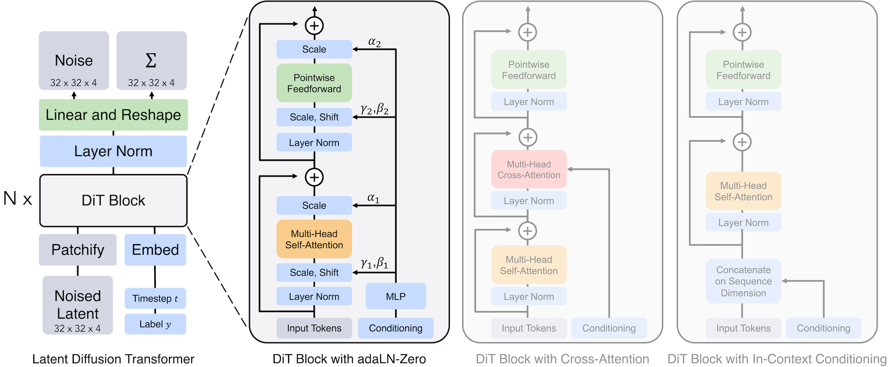
The first is standard cross-attention, which inserts the conditioning signal into each block with an additional attention mechanism. The second alternative is sequence concatenation, where the conditioning tokens are appended to the main sequence. We see the last approach used more and more in modern models like MMDiT (Multimodal Diffusion Transformer) [2], notably proposed in the Stable Diffusion 3 paper, where tokens of different modalities go through separate sets of weights.
Experiments
While DiT outperforms U-Nets, this was not the only takeaway message. The goal of [1] was to demonstrate that diffusion models based on transformers can scale as predictably as LLMs. To prove this, the authors conducted an extensive study across varying model configurations and compute resources.
In particular, they designed a grid of models defined by two main factors:
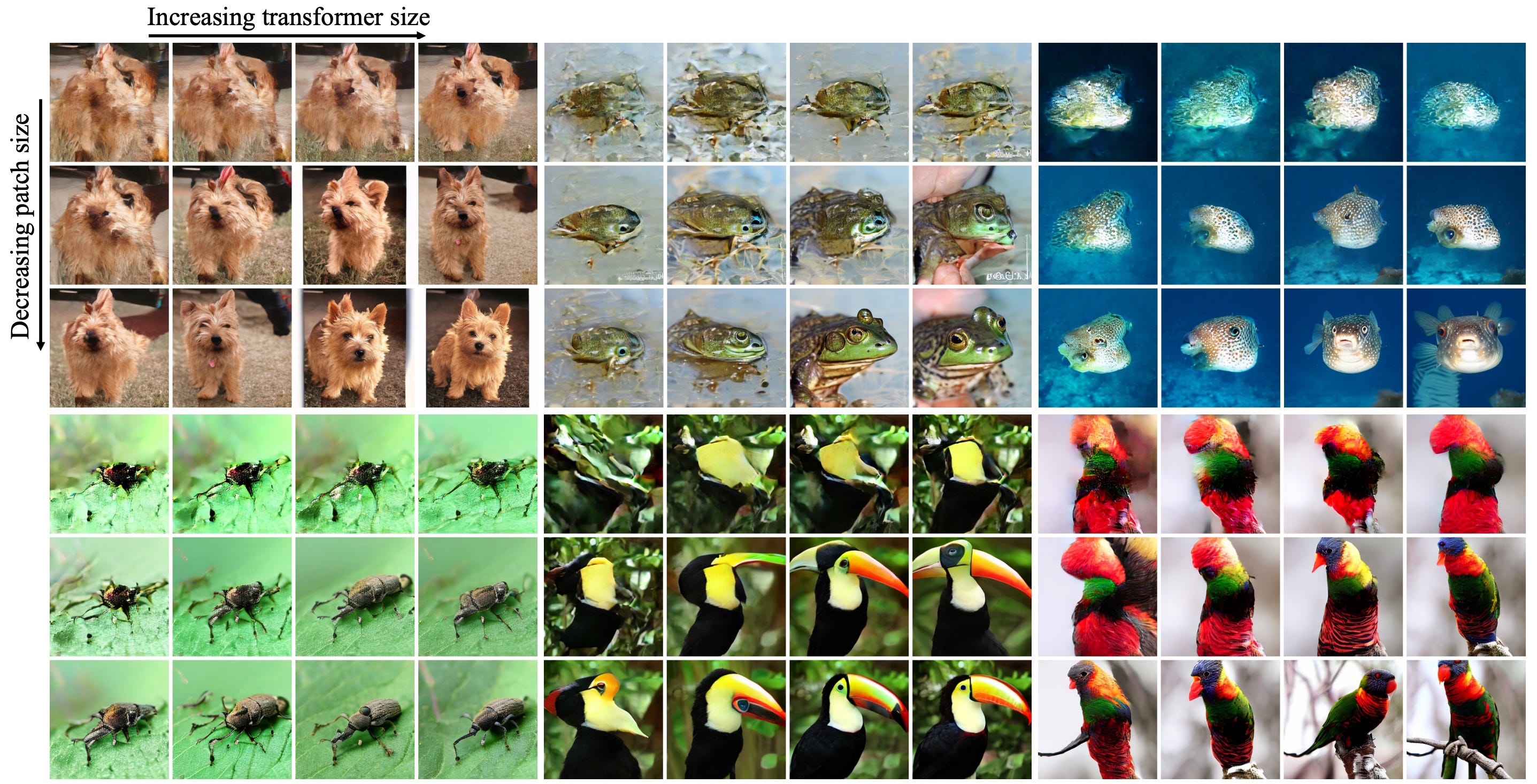
Model size. They ranged from small (DiT-S, 12 layers, embedding size 384) to extra large (DiT-XL, 28 layers, embedding size 1152). This controls the depth and width of the transformer, effectively determining the parameter budget.
Patch size. They tested patches of size 2, 4, and 8. This controls the sequence length and the granularity of information. A smaller patch size results in a longer sequence of tokens, but provides more room to store information.
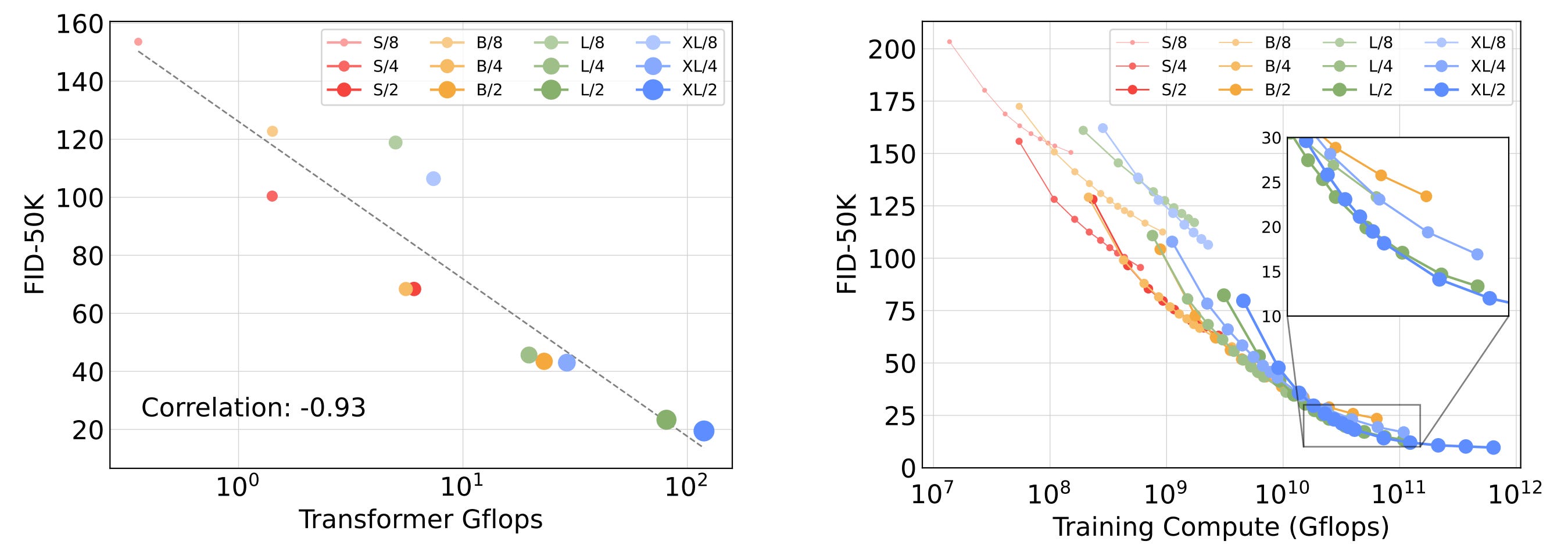
The results reveal that increasing the model size predictably improves performance. Similarly, decreasing the patch size yields better results. Furthermore, allocating more compute to the transformer during training leads to better images. In short, there are clear and predictable scaling laws, which is all that matters these days!
Conclusions
DiT shows that transformers are adaptable to generative modeling. With no surprise, they scale predictably similar to ViTs and LLMs. Furthermore, the design follows the “less is more” philosophy and adopts a general-purpose structure, fully embracing the idea that data dictates all the rules.
Today, Diffusion Transformers power plenty of state-of-the-art image and video generators (as well as the new wave of diffusion LLMs), so it is a fundamental building block to understand if you are into generative models. To name a few, we see variations of this in Stable Diffusion 3, FLUX, Qwen Image, and Sora. See you next week, and happy holidays!
References
[1] Scalable Diffusion Models with Transformers
[2] Scaling Rectified Flow Transformers for High-Resolution Image Synthesis