


6. Learning Visual Representations with SimCLR
A simple framework for contrastive learning


Introduction
As discussed in the previous article, self-supervised learning is a powerful approach to learning meaningful data representations without human-labeled data, allowing for seamless transfer to downstream tasks.
In computer vision, one of the most influential works in this space is SimCLR (Simple Framework for Contrastive Learning of Visual Representations) [1], introduced by Google Research in 2020. The title is no exaggeration — the idea behind it is remarkably simple. Let’s break down how it works.
Method
It all starts with a single image. Two independent sets of random augmentations — a sequence of random cropping with flipping, random color distortions, and random blur — are applied to it, generating two distinct views of the original.
These augmented views are then passed through the current neural network to obtain their respective embedding vectors, i.e. their numerical representations.
This procedure is repeated for multiple images in the dataset, generating two distinct views for each one and passing them through the neural network for encoding. With N images in a batch at this stage, we now have 2N representations, grouped in pairs.
The model is then trained to maximize the similarity between the embedding vectors of augmented views derived from the same image while minimizing their similarity to the embeddings of all other views in the batch, which serve as negatives. This results in N unique positive pairs and N(2N − 2) unique negative pairs per batch. Note how the negatives scale quadratically with the batch size.
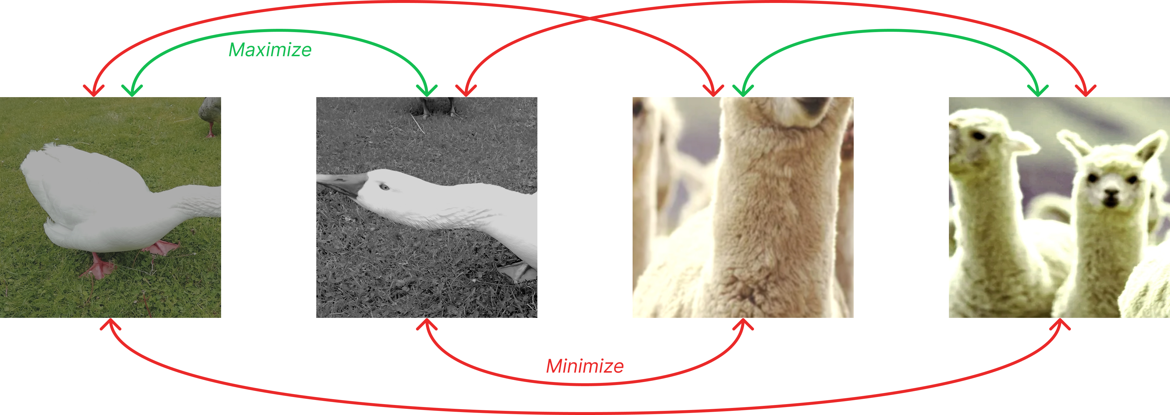
SimCLR relies on cosine similarity as the distance measure between vectors, which focuses on directional alignment in the feature space and ignores their magnitude, which naturally varies due to the diverse transformations applied.
And that’s pretty much it! This contrastive learning objective encourages the model to capture essential features that remain invariant across different transformations, leading to robust and transferable representations.
But as always, the devil lies in the details, and making this work requires some tricks, explained right below. But first, let’s recall standard evaluation protocols to test representation quality:
Full fine-tuning of the model weights with a classification layer on top
Linear probing, where we use the pretrained model as a frozen feature extractor and train only a classification head. This is used in all the plots below.
Making SimCLR effective
1) First, we need to add a projection head on top of the model, which is later discarded. In the paper, a ResNet-50 backbone is used, which produces a 2048-dimensional representation, and a 2-layer MLP projection head is attached to project this representation into a 128-dimensional space, where the loss is computed.
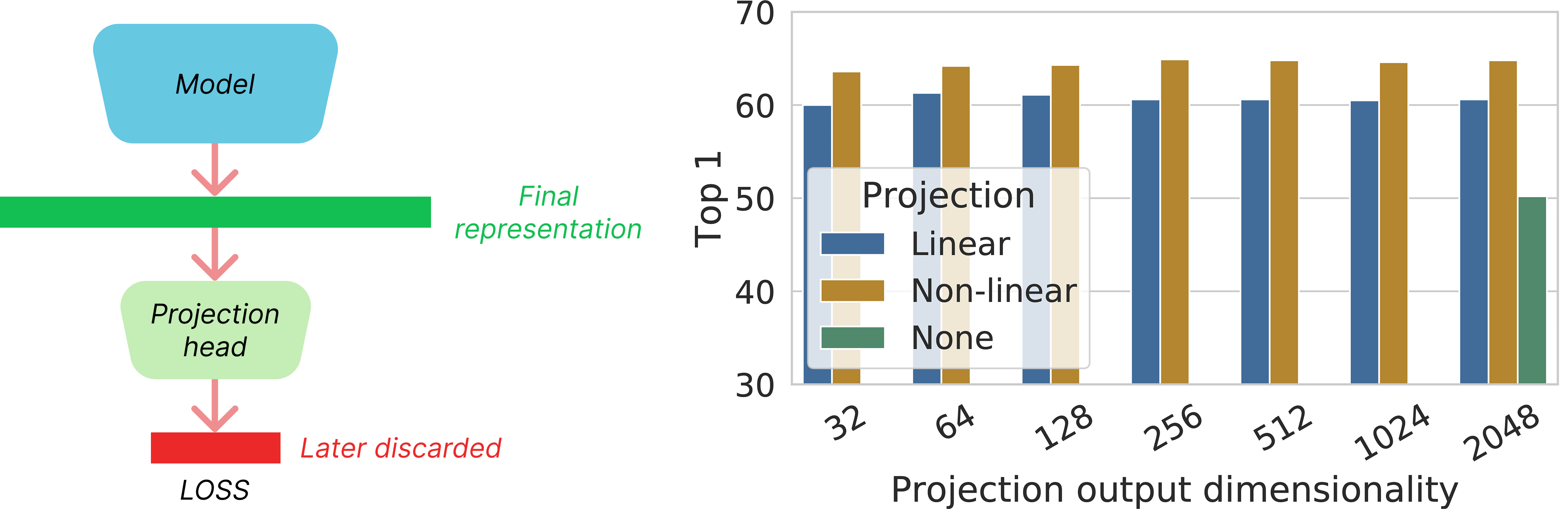
Experiments on task transfer show that a nonlinear projection is better than a linear projection (+3%), and much better than no projection (>10%), regardless of the output dimension. This is because the contrastive loss forces the final embeddings to be invariant to data transformations, potentially discarding information that could be useful for downstream tasks, such as the color or orientation of objects.
2) The second key point is that the approach is highly sensitive to the choice of augmentations. To demonstrate this, the authors performed a grid search over all possible pairs of augmentations and found that some combinations significantly outperform others. In particular, the best performance comes from combining cropping with color augmentations.
Cropping provides the strongest learning signal for capturing the semantics of an image (diagonal entries correspond to a single transformation, and the last column reflects the average over the row). Depending on the relative position of the two crops, the model needs to understand the relationship between disjoint but close views or relate global to local context, if one crop contains the other.

But why is color augmentation so important? Well, remember model shortcuts from the previous post? One of them lies here. The color distribution of pixels within crops of the same image is often very similar, and the model can use this fact to solve the task rather than truly understanding the content and looking at fundamental features.
Applying random color distortions to the crops prevents using this information, and forces the model to look at more relevant characteristics.
3) Finally, the model requires extremely large batch sizes during training, typically in the range of thousands of images. However, this is impractical for the average Joe to reproduce due to memory and computational constraints. Intuitively, with more negative examples available, the model can understand where not to place the embeddings in representation space, constraining the task more.

Another way of reading this figure is that training for longer leads to significant improvements. Also, using bigger networks improves performance, showing that scaling up all these aspects helps.
Conclusions
Despite the narrow range of requirements needed to make it work, the authors successfully implemented a simple framework for contrastive learning, demonstrating that a standard architecture is sufficient if the self-supervised task is meaningful.
SimCLR outperformed competing methods by a significant margin in downstream classification and paved the way for self-supervised pretraining to surpass supervised one, provided there is enough model capacity, the right set of data augmentations, and a projection head.
That being said, this exact sensitivity to augmentations and, most importantly, the necessity of large batch sizes are notable limitations. Additionally, there are problems connected to negative samples (for instance, two very similar images in the batch may be incorrectly treated as negatives), potentially leading to suboptimal representations.
We’ll see how future works address these challenges. Thanks for reading, and see you!
References
[1] A Simple Framework for Contrastive Learning of Visual Representations