8. Diffusion Models

Turning noise into realistic data, step by step

Introduction

Whenever you come across an incredibly realistic generated image, video, or audio, chances are a diffusion model was behind it. And if you didn’t notice, it probably worked a little too well.

This powerful and versatile class of generative models has surged in popularity not only because it can create high-quality samples, scale effectively, and be relatively easy to train but also due to its strong theoretical foundation rooted in physics and probability [1]. Today, we’ll take a closer look at how it all works, in a friendly manner.

The forward process: controlled destruction

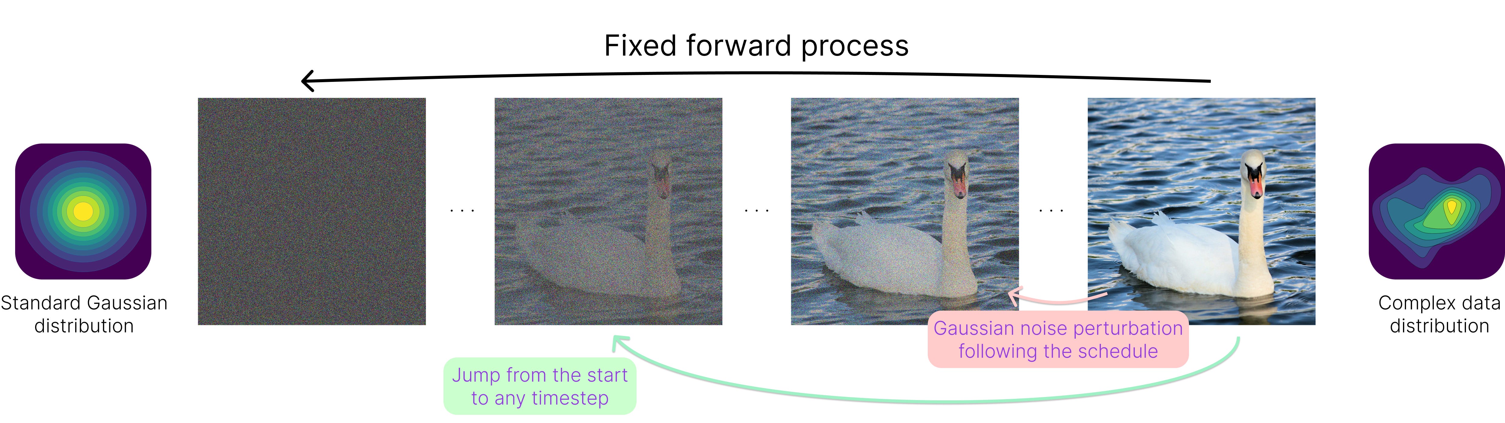
The forward process in diffusion models corrupts the data by progressively adding noise. This transformation occurs over multiple (e.g. 1000) steps, making the original data point less and less distinguishable until it becomes nearly pure randomness, much like uncarving a detailed sculpture back into a raw, shapeless block of marble.

The goal is to map any complex data distribution into a predictable one — typically a standard Gaussian distribution with mean 0 and variance 1 — with the property that every transition towards it is well-defined and the final state is easy to sample from, even in high dimensions.

In practice, using Gaussian noise perturbations for transitions is particularly convenient. Each new version of the noised data is obtained by taking a weighted average of the current state and a newly sampled Gaussian noise component. In this chain of operations, the structured noise addition ensures that the process remains mathematically tractable at all steps.

In the forward process, Gaussian noise is added to a data sample step by step until no structure is left.

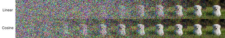
One aspect to highlight here is the presence of a noise schedule, which determines how much noise is added at each transition. Rather than applying noise uniformly, the schedule carefully controls the rate of corruption, determining how quickly the original data structure is lost. The higher the variance of a Gaussian perturbation, the quicker the convergence to pure randomness.

The linear schedule, which increases the variance linearly over time, is a popular choice [2]. However, a cosine-like schedule [3] is often preferred, as it slows down noise addition at early steps, helping preserve information for longer.

The cosine schedule adds noise more slowly at the beginning, preserving the signal for longer. Image from [3].

The second aspect to underline is that thanks to the properties of the Gaussian distribution, we can directly compute the noised data at any timestep using a closed-form equation, eliminating the need for step-by-step simulation.

In simple terms, one can “sum up all the perturbations” up to a certain point and express any intermediate noisy state as a function of the original data and a single Gaussian noise sample. By doing so, we can efficiently “jump” to any point in the forward process from the start, which is crucial for training as it eliminates the need to sequentially apply hundreds of operations to obtain a noisy sample.

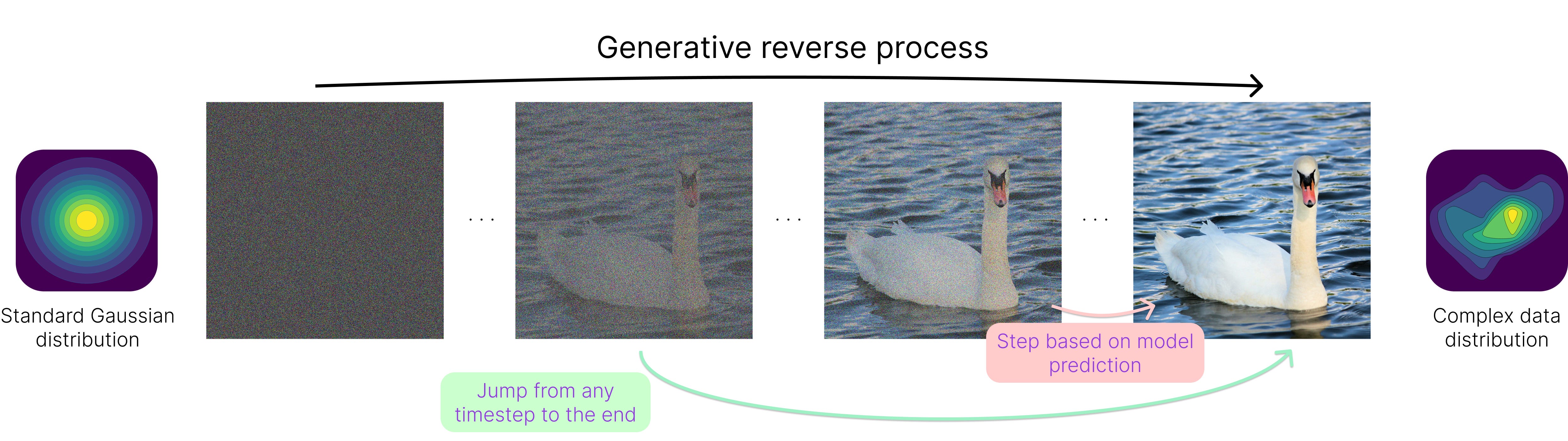
The reverse process: learning to denoise

As we just saw, creating noise from clean data is easy. The real challenge lies in the reverse process, where we must transform the initial standard Gaussian distribution back into the complex output distribution, unlocking the generative capabilities. Although this may sound almost impossible, it is achieved by training a neural network to remove noise step by step, given the current state and the noise schedule.

This slower progressive generation historically contrasts with other generative approaches such as GANs (Generative Adversarial Networks) and VAEs (Variational Autoencoders), which generate data in a single pass. However, it balances out with significantly better quality, diversity, and controllability in the generated outputs.

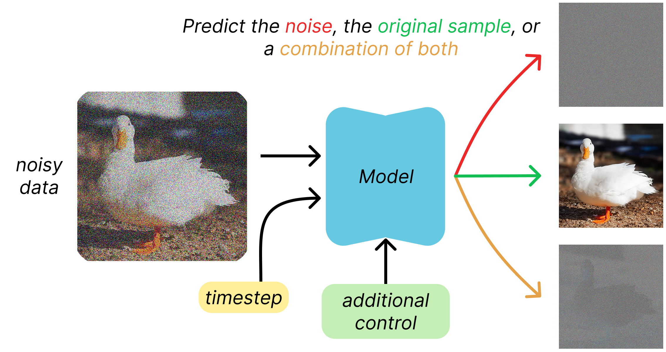
Thanks to the “jumping” property introduced before, given some clean data and a chosen timestep, we can generate a noisy training sample with a single operation, and we know everything about it. The model is then trained on the task of predicting either the noise that was added (ε-objective), the original clean sample (x0-objective), or a combination of both (v-objective). All these require predicting something with the same dimensionality as the input, and that is why architectures like U-Net are well-suited for diffusion models.

A single model is trained to reverse the noising process at all stages, given as input a noisy sample, the corresponding timestep, and optional extra conditioning. Different prediction objectives are possible.

Once the model is trained on a large and diverse set of original data samples combined with noise at different timesteps, it learns to effectively reverse the entire diffusion process. This means it can transform an initial Gaussian noise sample into a plausible output from the desired data distribution. That’s because it can predict and remove noise at various stages.

A point to make here is that similar to the forward process, one could “preview” the clean output at any point from the prediction. This means taking the direct output for a model trained with the x0-objective or applying simple transformations to the other predicted quantities.

The reason why it is not done in practice is that it generates coarse, low-quality outputs. It is like asking Michelangelo to carve the Pietà in one cut from a stone block instead of letting the artist patiently refine the sculpture.

Instead, we follow a reverse schedule, removing only a fraction of the noise at each timestep before estimating the clean signal again with the slightly denoised input. This approach allows for progressive refinement, ensuring that the generated output gradually converges to a high-quality, detailed sample rather than a rough approximation.

In the reverse process, we start with random noise. At each iteration, the model estimates the noise component and takes a corrective step in that direction, following the schedule.

There are ways to accelerate the generation to a much smaller fraction of the thousands of timesteps used in the forward pass (or even a single pass!), so this step-by-step approach is quickly becoming outdated. Still, a few steps are generally used.

Typically, the reverse process is not unconstrained (although it can be); rather, it is often conditioned on additional external information to guide generation, entering the realm of conditional diffusion models.

One example is text-conditional diffusion, where text embeddings from models like CLIP direct the generation process, as seen in Stable Diffusion. Another is image-conditional diffusion for tasks like inpainting, super-resolution, and even depth estimation. The condition is passed to the model alongside the current state and the timestep, as an additional input.

Conclusions

Diffusion models are widely adopted across different domains like image, video, and audio generation, but also in more vital fields like protein structure prediction and molecular generation in drug discovery. That’s because they are general: adding noise and learning to reverse it is a universal concept, independent of any data type (can even be done with text!).

With efficiency and sampling speed getting better every day, more fine-grained control mechanisms, and strong ongoing research and improvements, it seems like they are going nowhere in the near future. A promising alternative to map distributions seems to be flow matching, but I’ll talk about this in a future post.

If you are very technical and curious to dive deep into the mathematical foundations of diffusion, a good starting point is [4]. For code implementation, the plug-and-play gold standard is the Diffusers library by 🤗 Hugging Face [5].

Thanks for reading, and happy generation!

References

[1] Deep Unsupervised Learning using Nonequilibrium Thermodynamics

[2] Denoising Diffusion Probabilistic Models

[3] Improved Denoising Diffusion Probabilistic Models

[4] What are Diffusion Models?

[5] 🤗 Diffusers