
14. VQ-VAE: Vector Quantized Variational AutoEncoder
Learning discrete latent representations from raw data


Introduction
In the first article of the series, we talked about Variational Autoencoders (VAE) and discussed their ongoing relevance in modern machine learning systems. In short, VAEs learn efficient data representations in an unsupervised manner by mapping inputs into a continuous, lower-dimensional latent space and reconstructing them back. For a quick refresher (not essential, but helpful for following along), you can always read it here:

While modeling continuous variables in latent space is the biggest strength of VAEs, it also limits their scope to model classes that can effectively handle that continuous nature. Just to mention one, our beloved transformers are not on the list, which is quite the problem!
Vector Quantised-Variational AutoEncoders (VQ-VAEs) [1] represent the other side of the coin and come to the rescue by learning to embed the input data into discrete latent representations, opening new possibilities. Let’s dive in and see how they work.
Encoder, Decoder, and Codebook
At their core, VQ-VAEs still follow the standard autoencoder structure, so we have an encoder and a decoder responsible for compressing and decompressing the data. But here is the twist: between them lies the codebook, a learnable collection of K discrete embedding vectors that replaces the continuous latent space of traditional VAEs.

Made simple, the VQ-VAE takes an input, passes it through the encoder to produce a compressed latent representation, and then quantizes that representation by “rounding” each element to the nearest discrete vector in the codebook based on Euclidean distance. This discrete code is then passed to the decoder, which attempts to reconstruct the original input from it. As a result, we get a model that works with a finite set of K known representations, much like choosing words from a vocabulary.
Let’s consider a realistic example. Suppose we’re working with an image of size 256×256×3. This is first mapped into a latent space of size 32×32×16 using the encoder, trading spatial resolution for feature channels. Each 16-dimensional vector is then quantized by mapping it to the closest codebook element. This produces a quantized latent of the same shape, 32×32×16, which is then passed to the decoder to reconstruct the original 256×256×3 image. Remember that the beauty of an autoencoder is that it is trained in an unsupervised fashion, so no labeled data is required to achieve this!
Training the VQ-VAE
Getting a VQ-VAE to work well means optimizing all three of its main components: the encoder, the decoder, and the codebook. Intuitively, we want to both minimize reconstruction error as well as have a meaningful and well-utilized codebook.
But before we proceed, we need to address the elephant in the room, which is that the architecture is not end-to-end differentiable. Unlike VAEs, there is no clever reparameterization trick that can help here: the quantization step, where each encoder output is assigned to the nearest codebook vector, is a non-differentiable operation. This breaks the gradient path, and we can’t update the encoder and the codebook directly through this step.
To get around this, the VQ-VAE uses a technique called the straight-through estimator. During the backward pass, the gradients from the decoder are copied directly to the encoder output, bypassing the non-differentiable quantization step. This allows the encoder and decoder to be trained end-to-end, whereas the codebook is updated separately through its own loss.

Overall, there are three loss terms:
Reconstruction loss, which ensures the decoder accurately reconstructs the original data from the discrete codes. In the best-case scenario, despite working in this constrained discrete space, the codebook is large enough that we can have almost lossless compression and decompression. This term is also present in standard VAEs, but it is simplified since we no longer model a full probability distribution over the latent space (so no KL-divergence term).
Codebook loss, which pulls the selected codebook vectors toward the encoder outputs. This is a sparse loss, meaning it only affects the codebook entries that are chosen in the batch, and it basically helps the initial (random) codebook to adapt to the data distribution and become more expressive over time.
Commitment loss, which encourages the encoder to stick to using the codebook entries rather than drifting away or ignoring them. Without this symmetric term, the encoder might produce outputs that are too far from the nearest codebook entries, making quantization unstable. Due to the previous term, the codebook entries would also grow uncontrollably trying to follow them. This term is typically weighted with a constant beta.

As can be seen in the picture, both symmetric loss terms involve a stop-gradient operator, meaning we don’t update parameters during the backward pass for its argument, even though these are needed to compute the loss term. This way, in the end, both codebook entries and encoder parameters get updated, but they do so without interfering with each other.
From compression to generation
Like the VAE, its quantized counterpart VQ-VAE has also found numerous practical applications across diverse domains such as images, videos, and audio. On one side, discrete representations were already around in these domains long before deep learning, so these learned codebooks can extend existing tokenizers and compression methods.
On the other hand, they also have the advantage of being compatible with modern powerful models that operate over sequences, such as transformers. At the end of the day, the latent representation of a VQ-VAE is just a big tensor of categorical elements, and nothing is stopping us from modeling its distribution using an autoregressive model…
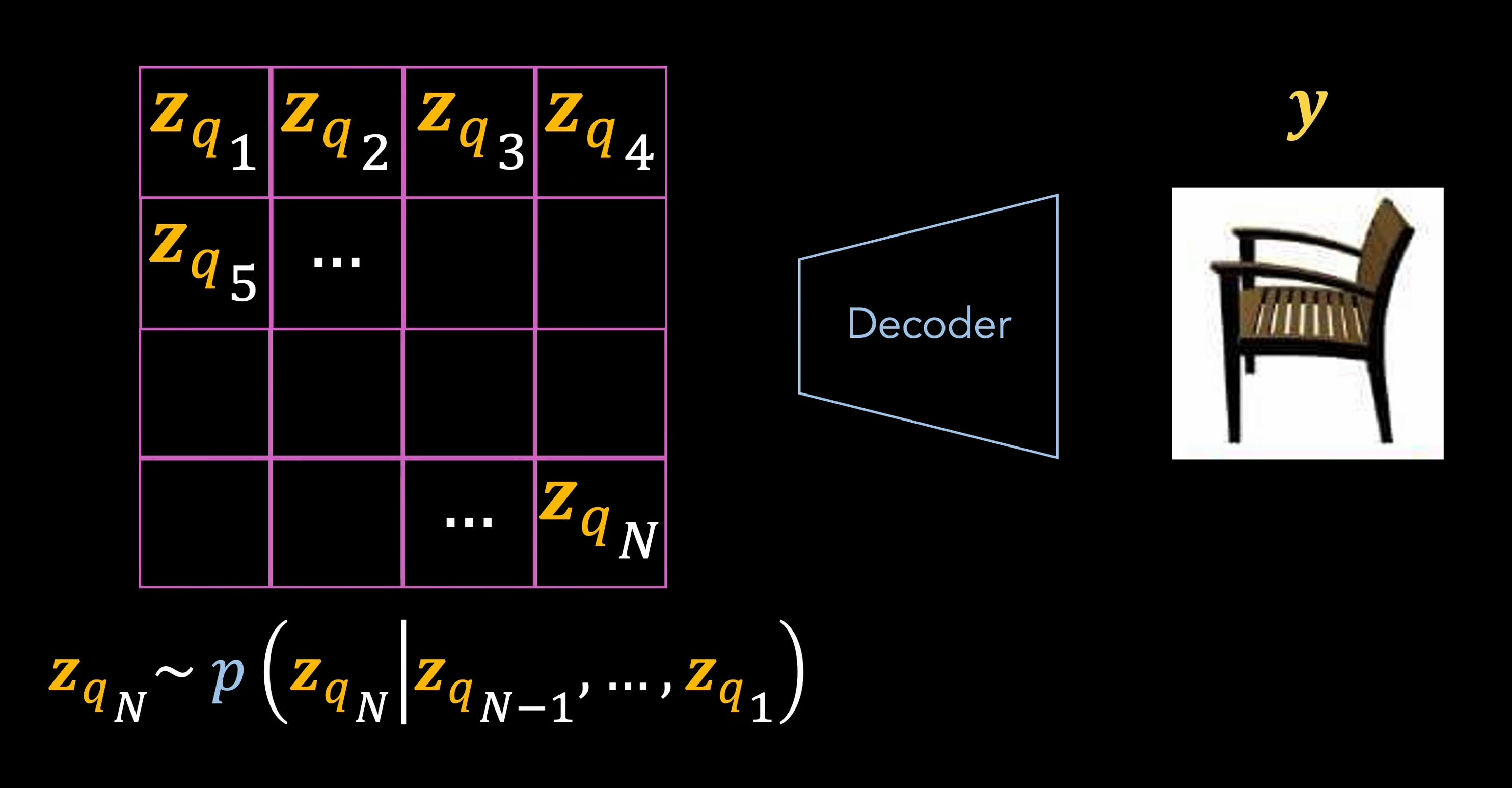
As the years have passed, we can argue that the VQ-VAE has proven to be especially impactful and versatile in generative modeling, as shown by several famous works, such as DALL·E (text-to-image), Jukebox (music generation), VQ-GAN (image synthesis), and many more.
Conclusion
The VQ-VAE takes the classic autoencoder framework and pushes it into the new territory of discrete latent spaces. Some challenges are posed by the non-differentiable quantization step, but they are nicely addressed by copying the gradients and a well-designed loss function. These are practical techniques worth remembering for your personal research or project work.
The second takeaway is that this framework is not only useful for compression but also suited for generative tasks, especially when paired with sequence models. We’ll dive into some of these works soon! As usual, it might be a bit hard to digest some of these topics, so I don’t mind sharing a good YouTube video that can help [2]. See you next week!
References
[1] Neural Discrete Representation Learning
[2] Vector-Quantized Variational Autoencoders (VQ-VAEs) from DeepBean