
25. Flow Matching
Efficient generative sampling via estimating velocity fields

Introduction
Diffusion models have dominated the generative landscape over the past four years with a formulation that is well-defined and modality-independent, coupled with a series of practical tricks that have made them scalable and efficient to sample from.
Generative modeling all boils down to mapping a simple distribution like a standard Gaussian to an arbitrarily complex data distribution. Once this is learned, new data can be generated by sampling from the simple Gaussian and applying the known mapping. Performing this complex transformation in one or a few steps is a task of major interest.
In diffusion, we learn to reverse a noisy stochastic trajectory, and as a result, approximating the sampling with very few steps is challenging. Thanks to more regular trajectories, Flow Matching [1] excels at this and is rapidly gaining traction as a better alternative to diffusion.
Today, we’ll look at similarities and differences between the two, actually concluding that they are pretty much two sides of the same coin, which is the best news for researchers and developers. Let’s go!
The probability flow
To understand flow matching, it’s helpful to introduce the continuous-time view of diffusion. As outlined in post #8, diffusion models are trained by applying a sequence of small, controlled noising steps for T times (e.g., 1000) until the signal is lost and the distribution is a standard Gaussian. At inference time, this process is then reversed.

The number T here is completely arbitrary, and the more we increase it, the more we approximate a continuous process that can be modeled via real numbers and a differential equation. This continuous process is what we would call a probability flow: a trajectory that smoothly transports probability mass from the complex data distribution to a simple Gaussian, and vice versa, defined for every value of t ∈ (0, 1).
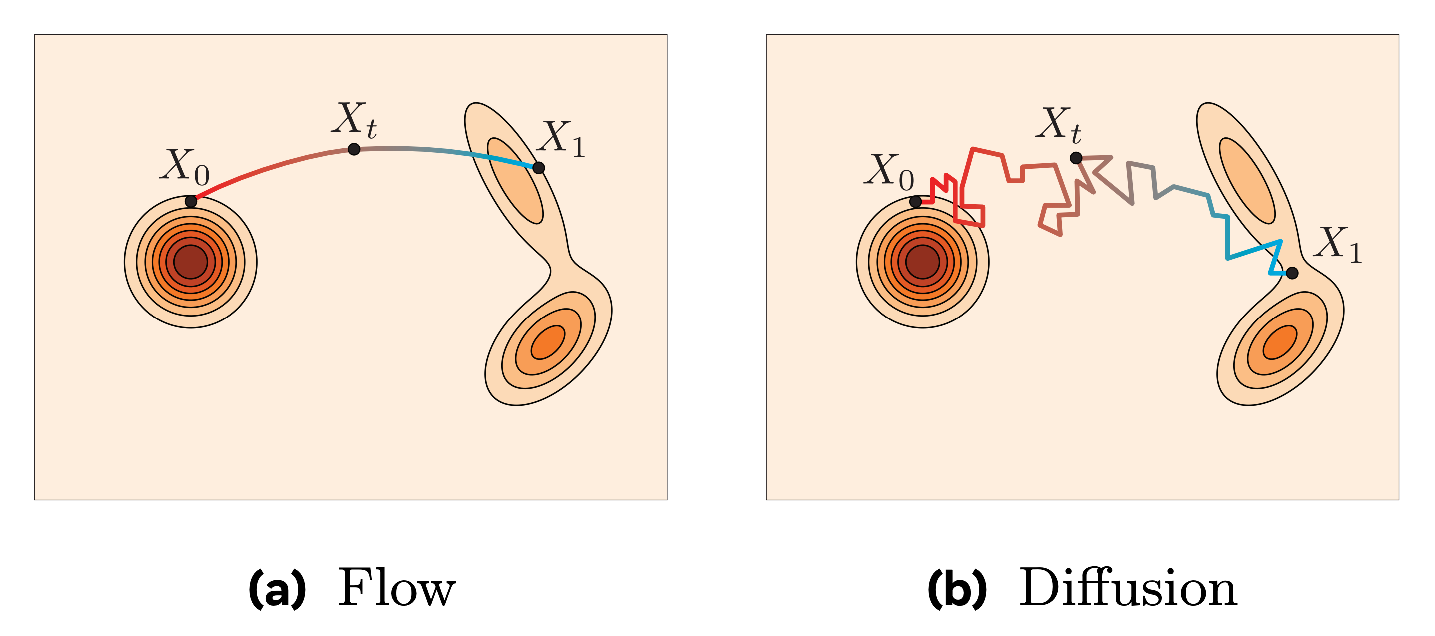
Now, in flow matching, we actually do the same thing in the forward pass! We keep it very simple, and adopt a smooth linear interpolation between the data and noise distributions, such that at time t ∈ (0, 1), we are modeling the variable z = (1 - t)x + tε. With some basic math, it can be shown that this corresponds to the diffusion forward process if the end noise ε is Gaussian and we adopt a particular schedule.
This means:
Both frameworks define a probability flow between a noise distribution and the data distribution.
Their forward processes can coincide analytically under certain boundary conditions. In general, diffusion uses a stochastic forward process, while flow matching typically relies on a deterministic one.
Learning algorithm
In diffusion, we train a model to predict the added noise (in the ε-objective) or some reparameterization of it, like the very popular v-objective. The model is supervised using the ground truth noise, derived analytically from the forward process, and trained via mean squared error.
Now, in flow matching, the learning objective is a bit different. Instead of predicting noise, we train a model to estimate the instantaneous velocity field that transports samples from the noise distribution to the data distribution over time. Think of it like learning the trajectory that deterministically moves samples from noise to data.
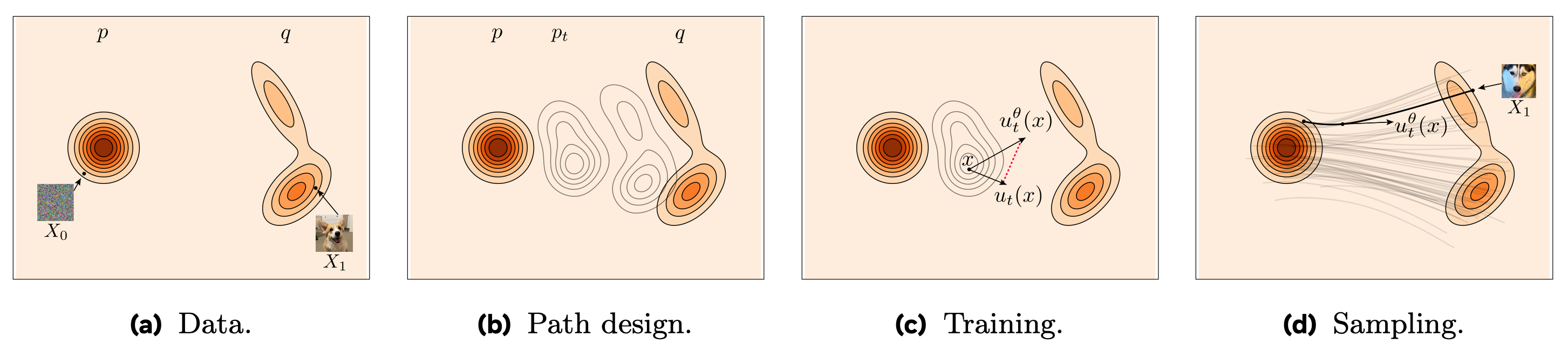
The setup works as follows: we sample a pair (x, ε), where x is a data point and ε is a noise sample, then linearly interpolate between them to obtain the interpolated point z = (1 - t)x + tε for a given time t ∈ (0, 1). The model is trained to predict the ground truth velocity at that point in time, i.e., the derivative of the interpolation path. This corresponds to the quantity v = ε - x, which is supervised via mean squared error too.
Crucially, in the linear interpolation setting between the two distributions, the path from x to ε moves at a constant “speed” in data space, so the instantaneous velocity field is the same for all t! This deterministic trajectory makes the learned model suitable for fast sampling via first-order solvers, and on top of this, it is also optimal in mathematical terms [1].
Once again, we can see some similarities:
Both frameworks perturb a clean sample via a forward process to produce noisy inputs, then train the model with an MSE loss to predict the “clean” signal (noise in diffusion, velocity in flow matching).
Since the input is always a perturbed sample, a time index t, and optional conditioning, they can share the same neural architectures. However, their training objectives differ, as explained.
Inference
To generate new data with diffusion, we first draw a sample from a standard Gaussian. Then, given the timestep t, we predict what the clean sample could look like with the model (we can always get that from any objective). With DDIM sampler, we perform a denoising step by projecting the estimated clean sample back to a lower noise level with the forward transformation. We keep alternating between predicting the clean sample and projecting it back to a lower noise level until completion.
To generate a new sample in flow matching, we again begin by drawing from a standard Gaussian. From there, we follow a deterministic trajectory guided by the learned velocity field. Basically, sampling reduces to numerically integrating backward from t=1 down to t=0 a simple differential equation that describes how to flow from noise to data. All we do is replace the vector field with our best guess at that time, and use a numerical solver to step.

In practice, since the model prediction approximates the theoretical constant velocity, the simplest update possible, z’ = z - v(z, t)Δt, works well even with relatively large Δt, yielding fast sampling! There’s no need for complex higher-order solvers, as a basic first-order (Euler) update, evaluated at a few steps along the unit interval, gets the job done fairly well.
Here are some more shared aspects:
In the sampling processes, both follow an iterative update that involves guessing the clean data at the current time step. In diffusion, we remove noise, while in flow matching, we predict velocity and move along it.
Running diffusion with DDIM sampler is the same as running the flow matching sampler with linear update. In both cases, we make the sampling loop fully deterministic.
Conclusions
If after reading all this you are still wondering what’s really different between diffusion and flow matching, I guess the answer is: nothing, they exhibit no fundamental differences, aside from training considerations and sampler choice.
However, if we had to highlight the contribution that Gaussian flow matching brings to the table, we would say it lies in the network output. Predicting the velocity field is arguably simpler to fit with a parametric model, and this can make a big difference in the training dynamics and scaling of these architectures.
Furthermore, flow matching is a more general framework: diffusion appears as a special case only when one uses Gaussian perturbations with a specific noise schedule. Technically speaking, flow matching allows for broader choices of forward and reverse paths, although there would be little reason not to use Gaussian noise and a straight linear interpolation for most cases…
If you want to dive deep into the math, something which I try to avoid most of the time in these posts, I can highly recommend the “Flow Matching Cookbook” [2] by Meta AI, the technical blog post “Diffusion Meets Flow Matching: Two Sides of the Same Coin” [3] by DeepMind researchers, as well as a Cambridge blog post [4].
As time passes, we already see major model releases shifting to this paradigm. Stable Diffusion 3 and Movie Gen by Meta AI, to name a few. So if you are into generative modeling, it's definitely worth updating your toolbox with this! See you next week.
References
[1] Flow Matching for Generative Modeling
[2] Flow Matching Guide and Code