
52. Pixel-Perfect Depth
Say goodbye to flying pixels in depth maps!

Introduction
The ability to perceive 3D structure from a single regular RGB image, also known as monocular depth estimation, is one of the most impressive features of the human visual system. While robots and autonomous vehicles operate with multiple cameras to make perception geometrically well-posed, monodepth remains necessary to protect against failure cases or to reconstruct 3D from already captured photos.
Lately, two approaches have been mainstream for solving the task. On one side, we can regress depth values on top of large-scale foundation models such as DINO. This discriminative approach involves aggregating features from multiple layers using a DPT decoder, and the most notable example in the community is undoubtedly the Depth Anything series [2, 3, 4].

The second, and much cooler, follows a generative paradigm, repurposing image diffusion models for dense prediction tasks. The prime example is Marigold [5], which leverages the massive world knowledge embedded in Stable Diffusion to generalize extremely well to in-the-wild images, but many others use even more recent models.
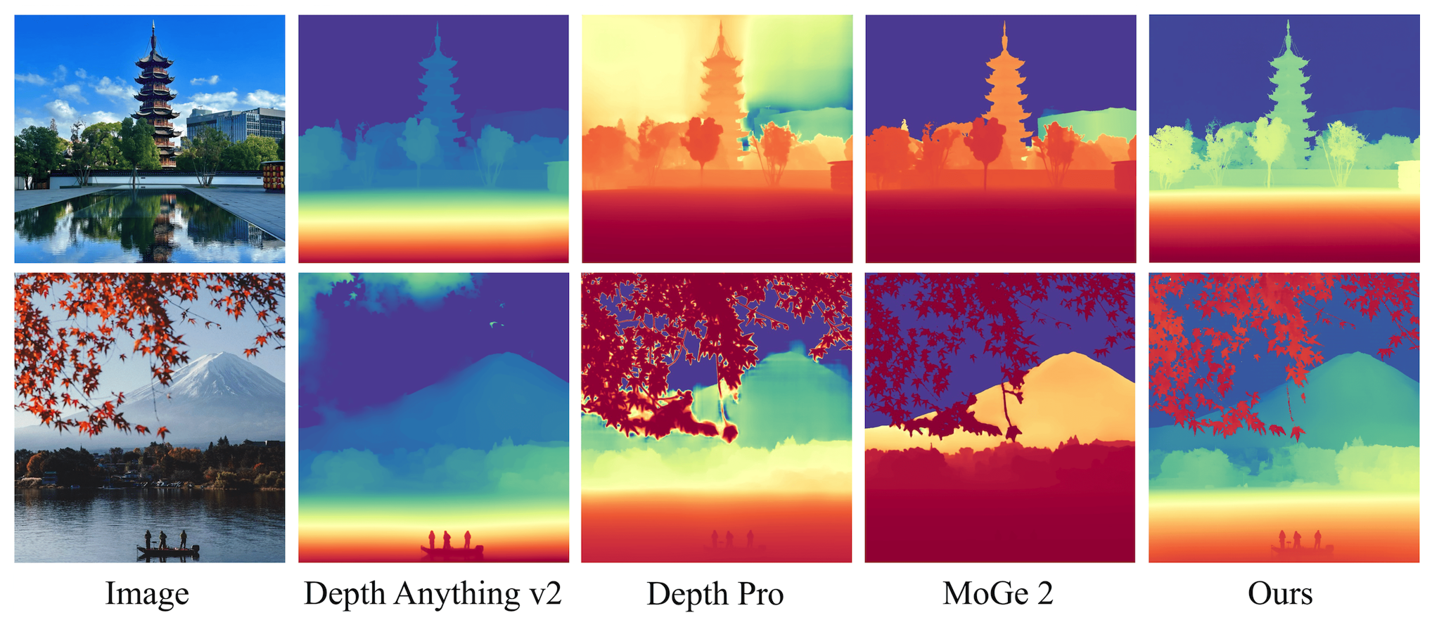
Choosing between the two paradigms depends on the specific use case and whether you prioritize high-frequency local details over global scene coherence. As you can imagine, the two ways keep exchanging the crown, but the goal is always to produce depth maps as sharp and accurate as possible. Today, we see a model that does just that: Pixel-Perfect Depth [1] (PPD), presented at the last NeurIPS.
The geometric failure of latent spaces
In generative depth estimation, practically all recent models use a latent diffusion process to keep computational costs manageable. This mirrors the widely successful strategy used in image generation, and is possible because pretrained Variational Autoencoders can work with normalized depth maps by treating them as grayscale images. All the details are explained in my previous post about Marigold, so if this doesn't make sense so far, go check it out!

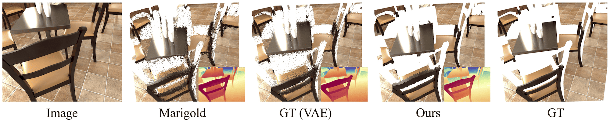
However, the main observation of PPD is that this lossy compression introduces a geometric bottleneck manifested as flying points at edges. In other words, the paper claims that latent diffusion-based backbones generate decently sharp depth maps, but the maximum quality is ultimately upper-bounded by the VAE itself. The easiest confirmation is the visual comparison here, where the GT after encoding and decoding — GT (VAE) — introduces flying points compared to the original GT.
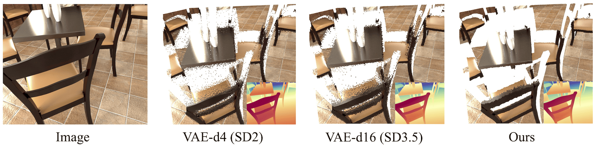
So, how can this be solved? Fighting the lossy nature of a VAE is hard, as the latent space is compressed overall by a factor of 12× to 48×. Modern VAEs (e.g., SD 3.5) are better, but still far from perfect. So, the authors take a radical approach and discard the VAE entirely, going back to pixel-space diffusion!
Method
Working in pixel space (or more accurately, patch space) allows modeling the depth distribution directly, including its discontinuities at object edges. However, training a Diffusion Transformer (#47) directly at high resolutions is computationally expensive and hard to optimize. To make this somehow tractable, PPD introduces two new components:
Cascade Diffusion Transformer. Instead of using a constant patch size for the whole network, it uses a coarse-to-fine strategy. For the first half of the DiT blocks, we have a larger patch size, significantly reducing the number of tokens to be processed. This also encourages the model to capture global image structures and low-frequency information early on.
In the second half of the layers, it switches to a patch size that is half as large, quadrupling the number of total tokens. This is done via an MLP that expands the hidden dimension by a factor of four, followed by a reshape. This second half shifts the focus to high-frequency details and refining boundaries. The patch sizes used in the two parts of the network are 16 and 8, with 12 DiT blocks each.
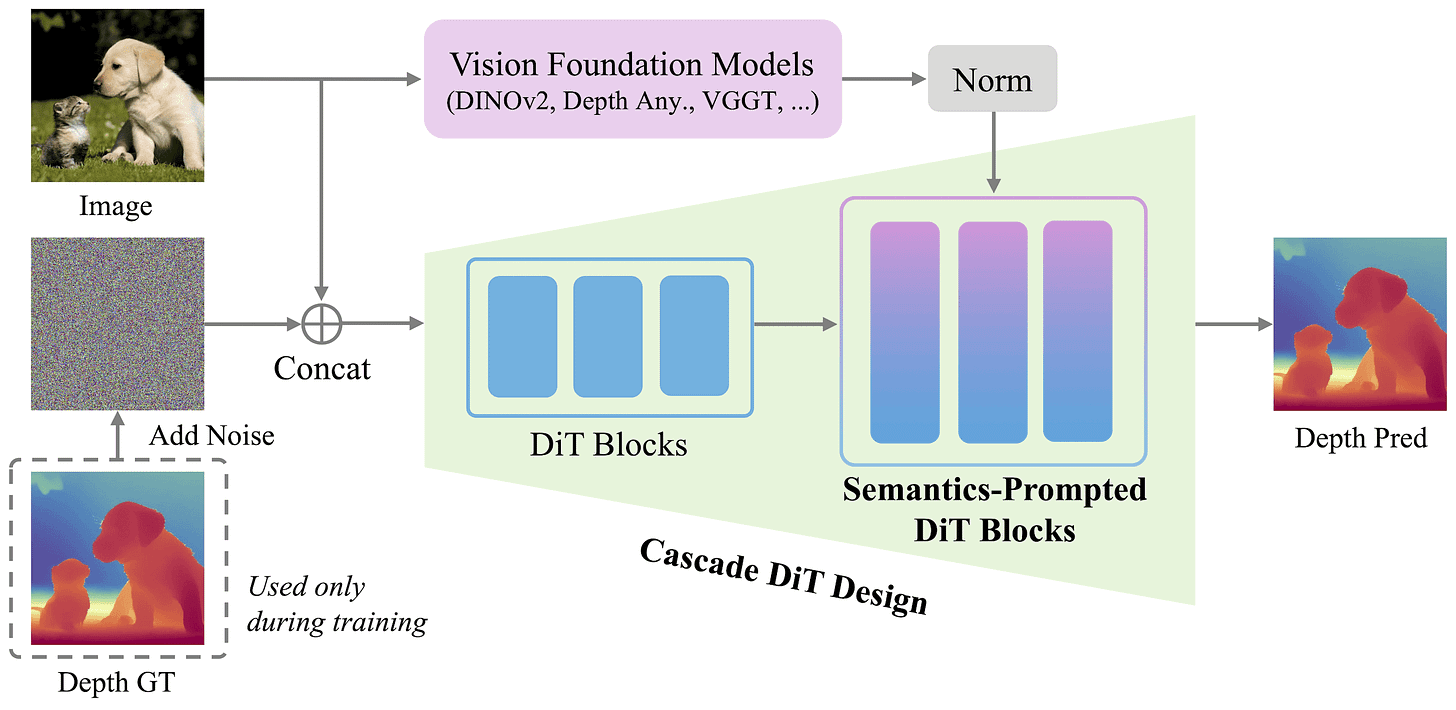
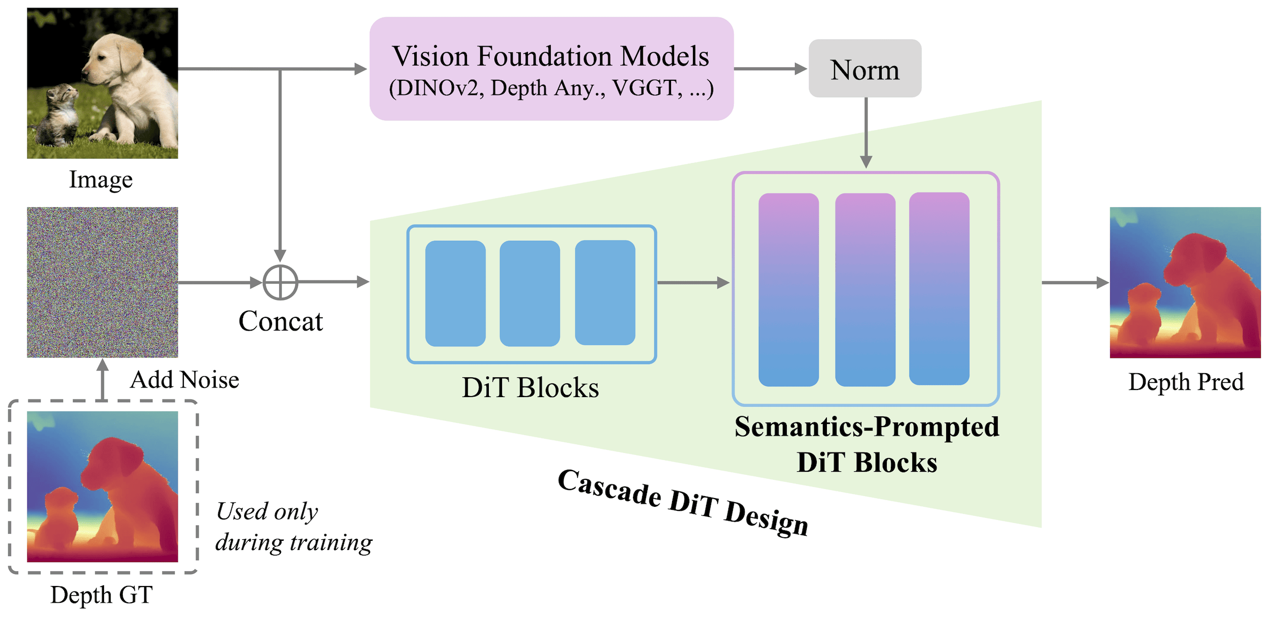
The cascade DiT in PPD switches patch size in the middle of the network. Architecture from [1]. Semantics-Prompted DiT (SP-DiT). The baseline design for a pixel-space DiT would concatenate RGB and noisy depth into a 4-channel input and produce a single-channel clean depth output (with patching & embedding at the start and unembedding & reassembly at the end). This strict RGB-noise concatenation induces spatial correspondence and mirrors the design of Marigold-like models. However, without the regularization of a structured VAE latent space, that alone isn’t enough to maintain global consistency with so many tokens, and the model ends up producing nonsensical geometry when we zoom out.
To fix this, the authors introduce the SP-DiT mechanism, which acts as a semantic compass for the diffusion process. In summary, it takes the input image and runs it through a frozen ViT encoder to extract high-level semantic representations (figure above). This can be a generalist one like DINO, or the fine-tuned ViT encoder from depth models like Depth Anything or VGGT. Because the magnitudes of these patch features may differ from those of the internal DiT tokens, the semantic representations are first normalized. Then, they are resized with bilinear interpolation to match the DiT patch size, concatenated channel-wise, and fused into the SP-DiT blocks via an MLP. In PPD, the first 12 blocks (the coarse stage) go without these prompts, while the remaining 12 blocks are SP-DiT blocks.
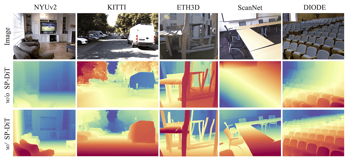
Despite being locally correct, plain DiT predictions would look nonsensical at the global level [1].

Training, evaluation, and video depth
As for the training strategy, the 500M-parameter model is first trained at 512×512 resolution on the Hypersim dataset, which consists of 54000 synthetic samples from interior scenes. The reason is that synthetic data provides perfect ground-truth labels free of sensor noise, which are necessary for fine-grained predictions in modern depth estimation models. Then, the input resolution is scaled up to 1024×768, and the model is fine-tuned using a mixture of five different datasets. Adding 70K outdoor samples is key to improving generalization in the real world.
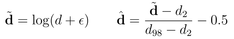
To ensure a more balanced capacity allocation across both indoor and outdoor scenes, the GT depth values are log-transformed and then scaled using the 2nd and 98th percentiles, following the normalization strategy in Marigold. The model is thus affine-invariant, but absolute metric depth can be recovered by leveraging external geometric foundation models providing scale and camera intrinsics. If that’s your application, you can find all the details in the GitHub codebase.
PPD is trained with the Flow Matching objective, which moves from predicting added noise to estimating a velocity field. This means that, for a sampled input noise ε and a clean depth x, the network is trained to predict the pixel-wise scalar quantity x-ε, which represents the straight path from noise to the data distribution. At training time, the noise level in [0,1] is sampled uniformly, so the model learns to denoise across all magnitudes. In inference, 4 equally spaced steps are used, and in these settings, it takes around 140ms on an RTX 4090.

A quick note on evaluating the flying points, maybe useful in interviews! Basically, the problem with standard depth metrics like AbsRel or RMSE is that they treat every pixel the same and are dominated by flat regions. To measure depth accuracy at edges, the paper extracts edge masks from the input using the Canny operator, and then computes the Chamfer Distance (a point cloud distance) between predicted and ground-truth clouds around these edges. The finding is that VAE-encoded-decoded depth has 50% higher error than PPD predictions, so the model produces significantly cleaner geometry than what a “perfect Marigold” would ever be capable of achieving.

As a last thing, for those interested in video, the authors also released Pixel-Perfect Video Depth (PPVD) last month, ensuring depth doesn’t flicker between frames and making it one of the best video depth models currently available. Check it out in the codebase https://github.com/gangweix/pixel-perfect-depth!
Conclusions
Pixel-Perfect Depth questioned the trend of latent-space predictions in monocular depth estimation, and shocked the community when it got a perfect (5,5,5,5) score at the last NeurIPS. By moving back to pixel space with a few tweaks, we finally have a way to generate depth maps that look clean while maintaining a fast runtime, which matters for real-world applications.
I recommend checking out the project page or the Hugging Face demo to inspect the point clouds. Enjoy exploring the results, and see you in the next one. By the way, these precise depth maps are also quite exciting for applications like 3D printing, in case you are into that!
References
[1] Pixel-Perfect Depth with Semantics-Prompted Diffusion Transformers
[2] Depth Anything: Unleashing the Power of Large-Scale Unlabeled Data
[4] Depth Anything 3: Recovering the Visual Space from Any Views
[5] Repurposing Diffusion-Based Image Generators for Monocular Depth Estimation